Coefficient for ω₂(x) = cosx/√π is \[ a_2 = \frac{1}{\sqrt{\pi}} \int _{-\pi}^{\pi} x\,\cos x\, {\text d}x = 0 \] again odd integrand.

Coefficient for ω₃(x) = sinx/√π becomes \[ a_3 = \frac{1}{\sqrt{\pi}} \int_{-\pi}^{\pi} x\,\sin x\, {\text d}x. \] Here the integrand is even, so \[ a_3 =\frac{2}{\sqrt{\pi}} \int_0^{\pi} x\,\sin x\, {\text d}x. \] Integrate by parts: \[ \int_0^{\pi} x\,\sin x\, {\text d}x = \left[ -x\cos x\right]_0^{\pi} + \int_0^{\pi} \cos x\, {\text d}x = \pi +0 = \pi . \] Thus, \[ a_3 =\frac{2}{\sqrt{\pi}}\cdot \pi = 2\,\sqrt{\pi} . \]

Apply Bessel’s inequality \[ \sum _{n=1}^{\infty }|a_n|^2\leq \| f\| ^2. \] Let’s compute both sides. The left-hand side (partial sum) is \[ |a_1|^2+|a_2|^2+|a_3|^2 =0+0+4\pi = 4\pi \approx 12.5664 . \] the right-hand side: the norm of f(x) = x \[ \| f\|^2 = \int_{-\pi}^{\pi} x^2\, {\text d}x = 2\int_0^{\pi} x^2\, {\text d}x = \frac{2\,\pi ^3}{3} \approx 20.6709 . \] Compare numerical values, we conclude that \[ 4\pi \leq \frac{2\pi^3}{3}, \] which confirms Bessel’s inequality.

What this example shows:

Even if we take only one nonzero coefficient (𝑎₃ = 2√π), the sum of squares \[ |a_3|^2=4\pi \] is already bounded above by the total energy ∥ f ∥² ≈ 20.6709. Adding more orthonormal functions can only increase the left-hand side, but it can never exceed ∥ f ∥². This illustrates the geometric meaning: the squared lengths of the projections of f onto any orthonormal system cannot exceed the squared length of f itself.    ■

Parseval's identity for the complex Fourier series states that the average power of a periodic signal is equal to the sum of the squared magnitudes of its complex Fourier coefficients. It equates the time-domain energy over one period to the frequency-domain representation: \[ \frac{1}{T} \int_0^T |f(t)|^2 {\text d}t = \mbox{V.P.} \sum_{n=-\infty}^{\infty} \left\vert c_n \right\vert^2 , \quad c_n = \frac{1}{T} \int_0^T f(t)\,e^{-{\bf j} 2\pi nt/T} {\text d}t . \]

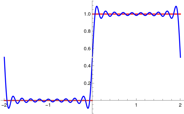
Example: We consider the Heaviside function: \[ H(t) = \begin{cases} 1, &\quad\mbox{for } t > 0, \\ \frac{1}{2} , &\quad\mbox{for } t =0 , \\ 0, &\quad\mbox{for } t < 0. \end{cases} \] Using Mathematica we evaluate the Fourier coefficients

Legendre polynomials    can be defined by Rodrigues' formula: \[ P_n (x) = \frac{1}{2^n n!}\,\frac{{\text d}^n}{{\text d} x^n} \left( x^2 -1 \right)^n = \frac{1}{2^n} \sum_{k=0}^{\lfloor n/2 \rfloor} (-1)^k \binom{n}{k} \binom{2n-2k}{n} x^{n-2k} , \] or via recurrence \[ \begin{split} \left( n+1 \right) P_{n+1} (x) &= \left( 2n+1 \right) x\,P_n (x) -n\,P_{n-1} (x) , \qquad n=1,2,\ldots , \\ P_0 (x) &= 1, \qquad P_1 (x) = x , \quad P_2 (x) = \frac{1}{2} \left( 3 x^2 -1 \right) . \end{split} \] A function f from Hilbert space 𝔏²([−1,1]) can be expanded into Fourier--Legendre series with respect to Legendre polynomials \[ f \,\sim\, \sum_{n\ge 0} a_n P_n (x) , \qquad a_n = \left( n + \frac{1}{2} \right) \cdot c_n , \quad c_n = \int_{-1}^1 f(x)\,P_n (x)\,{\text d} x . \tag{L.1} \] Parseval's identity: \[ \| f(x) \|^2 = \int_{-1}^{+1} | f(x) |^2 {\text d} x = \sum_{n\ge 0} \left( n + \frac{1}{2} \right)^{-1} a_n^2 = \sum_{n\ge 0} \left( n + \frac{1}{2} \right) c_n^2 . \tag{L.2} \]

Example: We apply Legendre expansion (L.1) to f(x) = xⁿ. Because monomial xⁿ and Legendre's polynomial Pₖ(x) have definite parity, only terms with the same parity as n, the Legendre coefficients appear also in the same parity. \[ x^n = \sum_{k=0}^n a_k P_k (x) , \qquad a_k = \left( k + \frac{1}{2} \right) c_k, \quad c_k = \int_{-1}^1 x^n P_k (x)\,{\text d}x , \] where \[ a_k = \frac{(2k+1)\, n!}{(n-k)!!\, (n+k+1)!!},\qquad n-k\ \mathrm{even}. \]

Here is Mathematica's code for evaluation of coefficients in the Legendre expansion:

Chebyshev expansions:   

The Chebyshev expansion of a function f ∈ 𝔏²([−1, 1], w dx) is its series representation of the form (that converges in the norm of the Hilbert space) \[ f(x)\sim \sum _{n=0}^{\infty }a_n\, X_n(x), \] where Xₙ is one of Chebyshev polynomials: Tₙ, Uₙ, Vₙ, or Wₙ. These polynomials were first presented by the Russian scientist Pafnuty Chebyshev in a paper read before the St. Petersburg Academy in 1853.

Parseval's identity corresponding to Chebyshev expansions always has the form \[ \| f(x) \|^2 = \int _{-1}^1|f(x)|^2 w(x)\, {\text d}x = \sum _{n=0}^{\infty} a_n^2\, \| X_n\| ^2, \] where ∥ Xₙ ∥² is the squared norm of the polynomial under its weight.

Chebyshev polynomials of the first kind are defined on interval [−1,1] by the formula \[ T_n (\cos\theta ) = \cos \left( n\,\theta \right) \] or by recurrence \[ \begin{split} T_{n+1} (x) &= 2x\,T_n (x) - T_{n-1} (x) , \qquad n=1,2,\ldots , \\ T_0 (x) &= 1, \qquad T_1 (x) = x , \quad T_2 (x) = 2 x^2 -1 . \end{split} \] or via the Jacobi polynomials \[ T_n (x) = \frac{P_n^{(-1/2, -1/2)} (x)}{P_n^{(-1/2, -1/2)} (1)} = \frac{2^{2n} \left( n! \right)^2}{(2n)!}\, P_n^{(-1/2, -1/2)} (x) . \]

Example: We want to expand the monomial xⁿ into the Fourier--Chebyshev series with respect to the Chebyshev polynomials of the first kind: \[ x^n = \frac{1}{2}\, c_{n,0} + \sum _{k=1}^n c_{n,k}\, T_k (x), \tag{T.3} \] where \[ c_{n,k} = \frac{1}{2^{n-1}} \binom{n}{(n - k)/2} \] Because upon substitution x = cosθ into manomial \( \displaystyle \ x^n =\cos^n \theta \ \) has definite parity, only terms with the same parity as n appear in expansion (T.3). Since Chebyshev expansions for monomials xⁿ with odd n involve T₀ ≡ 1 whose norm is different from norms of other Chebyshev polynomials, the corresponding Parseval's identity reflects this situation similarly to the classical trigonometric Fourier series.

Chebyshev polynomials of the second kind are defined on interval {−1,1} by the formula \[ U_n (\cos\theta ) = \frac{\sin \left( n+1 \right) \theta}{\sin\theta} \] or by recurrence \[ \begin{split} U_{n+1} (x) &= 2x\,U_n (x) - U_{n-1} (x) , \qquad n=1,2,\ldots , \\ U_0 (x) &= 1, \qquad U_1 (x) = 2x , \quad U_2 (x) = 4 x^2 -1 . \end{split} \] or via Jacobi polynomials \[ U_n (x) = \left( n+1 \right) \frac{P_n^{(1/2, 1/2)} (x)}{P_n^{(1/2, 1/2)} (1)} = \left( n+1 \right) \frac{n!\,\Gamma \left( \frac{3}{2} \right)}{\Gamma \left( n + \frac{3}{2} \right)}\, P_n^{(1/2, 1/2)} (x) = \left( n+1 \right) \frac{n! 2^n}{\left( 2n+1 \right) !!}\, P_n^{(1/2, 1/2)} (x) . \] Any function f ∈ 𝔏²([−1, 1], w dx) can be expanded into convergent Chebyshev series \[ f \,\sim\, \sum_{k\ge 0} a_{k} U_k (x) , \tag{U.1} \] where 𝑎ₖ = ⟨ f∣Uₖ ⟩, and the inner product in Hilbert space 𝔏³_w is \[ \langle f \mid g \rangle = \int_{-1}^1 f(x)\,g(x)\,w(x)\,{\text d}x , \quad w_U (x) =\sqrt{1-x^2}. \] The norms of Chebyshev polynomials of the second kind are all the same for any index: \[ \| U_n\| ^2 = \int_{-1}^1 U_n^2 (x)\,\sqrt{1-x^2}\,{\text d}x = \frac{\pi }{2}. \] Parseval identity: \[ \| f \|^2 = \int_{-1}^1 f^2 (x)\,U_n (x) \,\sqrt{1-x^2}\,{\text d}x = = \frac{\pi}{2} \sum_{k\ge 0} a_{k}^2 . \tag{U.3} \]

Example: We are looking for expansions of monomials xⁿ with respect to Chebyshev polynomials of the second kind \[ x^n = \sum_{k=0}^n a_{n,k} U_k (x) , \] where \[ a_{n,k} = \frac{1}{2^n} \left[ \binom{n}{n - k)/2} - \binom{n}{(n - k - 2)/2} \right] . \tag{U.2} \] Mathematica helps to determine these coefficients:

Chebyshev polynomials of the third kind are defined by the formula \[ V_n (\cos\theta ) = \frac{\cos \left( n + \frac{1}{2} \right)\theta}{\cos\left( \frac{\theta}{2} \right)} \] or by recurrence \[ \begin{split} V_{n+1}(x) &= 2x \, V_n(x) - V_{n-1}(x) , \qquad n = 1,2,\ldots , \\ V_0 (x) &= 1 , \quad V_1 (x) = 2x - 1, \quad V_2 (x) = 4 x^2 - 2x -1 . \end{split} \] or through Chebyshev polynomials of the first and second kinds \[ V_n (x) = T_n (x) + \left( x-1 \right) U_{n-1}(x) , \qquad n=1,2,\ldots , \] or via Jacobi polynomials \[ V_n (x) = \frac{P_n^{(-1/2, 1/2)}(x)}{P_n^{(-1/2, 1/2)}(1)} = \frac{4^n \left( n! \right)^2}{(2n)!}\,P_n^{(-1/2, 1/2)}(x) . \] Let ℌ = 𝔏²_w ≡ 𝔏²([−1,1], w dx) be the (real) Hilbert space, equipped with the inner product \[ \langle f \mid g \rangle = \int_{-1}^1 f(x)\,g(x)\,w(x)\,{\text d} x , \quad w_V(x) = \frac{\sqrt{1+x}}{\sqrt{1-x}} . . \] Chebyshev polynomials of the third kind Vₙ form an orthogonal system in the Hilbert space ℌ = 𝔏²([−1, 1], w dx) with weight \[ w(x) = (1 - x)^{-1/2} \cdot (1 + x)^{1/2} = \sqrt{\frac{1+x}{1-x}} . \] Any function f from ℌ can be extended into convergent (in the norm of the Hilbert space) series over Chebyshev polynomials of the third kind: \[ f (x) = \sum_{n\ge 0} b_n V_n (x) , \] where \[ b_n = \frac{\langle f \mid V_n \rangle}{\langle V_n \mid V_n \rangle} = \frac{1}{\pi}\,\langle f \mid V_n \rangle = \frac{1}{\pi}\,\int_{-1}^1 f(x)\,V_n (x)\,\sqrt{\frac{1+x}{1-x}}\,{\text d} x \] because norms of all Chebyshev polynomials of the third kind are the same, \[ \| V_n\|^2 = \int_{-1}^1 V_n^2 (x)\,\sqrt{\frac{1+x}{1-x}}\,{\text d} x = \pi , \quad n=0,1,2,\ldots . \] Then Parseval identity will be as follows: \[ \frac{1}{\pi}\, \| f \|^2 = \frac{1}{\pi}\, \int_{-1}^1 f^2 (x)\,\sqrt{\frac{1+x}{1-x}}\,{\text d}x = \sum_{n\ge 0} b_n^2 . \]

Example: We consider expansion of monomials xⁿ into series with respect to Chebyshev polynomials of the third kind \[ x^n = \sum_{k=0}^n b_{n,k} V_n (x) , \] where \begin{align*} \pi\,b_{n,k} &= \langle x^n \mid V_k \rangle = \langle x^n \mid T_k \rangle + \langle x^n \mid \left( x-1 \right) U_{k-1} \rangle \\ &= \langle x^n \mid T_k \rangle + \langle x^{n+1} \mid U_{k-1} \rangle - \langle x^n \mid U_{k-1} \rangle \\ &= \frac{1}{2^{n-1}} \binom{n}{(n-k)/2} + \frac{1}{2^{n+1}} \left[ \binom{n+1}{(n-k)/2} - \binom{n+1}{(n-k-2)/2} \right] \\ &\quad - \frac{1}{2^n} \left[ \binom{n}{(n-k-1)/2} - \binom{n}{(n-k-3)/2} \right] \end{align*} We can let Mathematica do these integrals symbolically.

Chebyshev polynomials of the fourth kind are defined by the formula \[ W_n (\cos\theta ) = \frac{\sin \left( \frac{2n+1}{2}\,\theta \right)}{\sin \left( \frac{\theta}{2} \right)} = \sum_{k = \lceil n/2 \rceil}^n \binom{k}{n-k} 2^{2k-n-1} (-1)^{n-k} x^{2k-n-1} \left( 2x +2 - \frac{n}{k} \right) , \quad n\ge 2, , \qquad x= \cos\theta , \qquad n=0,1,2,\ldots . \] or by recurrence \[ \begin{split} W_{n+1} (x) &= 2x\, W_n (x) - W_{n-1} (x) , \\ W_0 (x) &= 1, \quad W_1 (x) = 2x+1 , \quad W_2 (x) = 4x^2 + 2x -1 . \end{split} \] or through Chebyshev polynomials of the second kind \[ W_n (x) = U_n (x) + U_{n-1} (x) , \qquad n=1,2,\ldots . \]

Chebyshev polynomials of the fourth kind form an orthogonal system in Hilbert space ℌ = 𝔏²_w ≡ 𝔏²([−1,1], w dx), with weight \[ w_W (x) =\frac{\sqrt{1-x}}{\sqrt{1+x}} . \] These polynomials all have the same norm: \[ \| W_n\|^2 = \int_{-1}^1 W_n^2 (x) \,\sqrt{\frac{1-x}{1+x}} \,{\text d}x = \pi , \qquad n=0,1,2,\ldots . \] Then any function f from ℌ can be expanded into convergent in the norm series \[ f(x) = \sum_{n\ge 0} b_n W_n (x) , \qquad b_n = \frac{1}{\pi}\,\int_{-1}^1 f(x)\,W_n (x)\,\sqrt{\frac{1-x}{1+x}} \,{\text d}x . \tag{W.1} \] Parseval identity: \[ \frac{1}{\pi}\,\| f \|^2 = \frac{1}{\pi}\,\int_{-1}^1 f^2 (x)\,\sqrt{\frac{1-x}{1+x}}\,{\text d}x = \sum_{n\ge 0} b_n^2 . \tag{W.2} \]

Example: We are looking for expansions of monomials xⁿ with respect to Chebyshev polynomials of the fourth kind \[ x^n = \sum_{k=0}^n b_{n,k} W_k (x) , \] We can let Mathematica do these integrals symbolically.

Laguerre polynomials    were invented and studied by Pafnuty Chebyshev in 1859. Therefore, these polynomials were known in nineteen century as Chebyshev--Laguerre polynomials. There is no evidence that Edmond Laguerre (1834–1886) used them.

Laguerre polynomials can be defined by the Rodrigues formula, \[ L_n (x) = \frac{e^x}{n!}\,\frac{{\text d}^n}{{\text d} x^n} \left( e^{-x} x^n \right) = \sum_{k=0}^n \binom{n}{k} \frac{(-1)^k}{k!}\, x^k , \] or recurrence relation \[ \begin{split} \left( n+1 \right) L_{n+1} (x) &= \left( 2n+1 -x \right) L_n (x) -n\, L_{n-1} (x) , \qquad n=1,2,\ldots , \\ L_0 (x) &= 1, \quad L_1 (x) = 1- x , \quad L_2 (x) = \frac{1}{2} \left( x^2 -4x +2 \right) . . \end{split} \] The Laguerre polynomials are orthogonal on [0, ∞) with weight w: \[ \int _0^{\infty } L_m(x)\,L_n(x)\,e^{-x}\, {\text d}x =\delta _{mn}. \] For any function f ∈ 𝔏²([0,∞), e^−xdx), its Laguerre expansion becomes \[ f(x)\sim \sum _{n=0}^{\infty }a_n\, L_n(x), \] with coefficients \[ a_n =\int _0^{\infty } f(x)\, L_n(x)\, e^{-x}\, {\text d}x. \] Because the system is orthonormal, Parseval takes the simplest possible form: That’s the entire identity — no extra factors, because the classical Laguerre polynomials are already normalized in 𝔏²([0,∞), e^−xdx). \[ \| f \|^2 = \int_0^{\infty} |f(x)|^2 e^{-x}{\text d} x = \sum_{n\ge 0} a_n^2 , \qquad a_n = \int_{0}^{\infty} f(x)\,L_n (x)\, e^{-x} {\text d}x . \]

Example: The monomial xⁿ has the finite expansion \[ x^n\; =\; n!\, \sum _{k=0}^n (-1)^k {n \choose k}\, L_k(x). \] So the coefficient of Lₖ(x) is \[ a_{n,k} =n!\, (-1)^k {n \choose k},\qquad k=0,1,\dots ,n. \] You can check quickly with Mathematica:

The "physicist's Hermite polynomials" are given by the Rodrigues formula, \[ H_n (x) = (-1)^n e^{x^2} \frac{{\text d}^n}{{\text d} x^n}\, e^{-x^2} \] or recurrence relation \[ \begin{split} H_{n+1} (x) &= 2x\, H_n (x) - 2n\, H_{n-1} (x) , \qquad n=1,2,\ldots , \\ H_0 (x) &= 1, \quad H_1 (x) = 2x, \quad H_2 (x) = 4x^2 -2 . \end{split} \] The orthogonality relation \[ \int _{-\infty }^{\infty }H_m(x)H_n(x)e^{-x^2}\, {\text d}x = 2^n n!\sqrt{\pi}\, \delta _{mn} \] tells us that the ordered system of Hermite polynomials { Hₙ(x) }_n≥0 forms an orthogonal basis in Hilbert space ℌ = 𝔏²(ℝ, w dx)), equipped with the inner product \[ \langle f \mid g \rangle = \int_{-\infty}^{\infty} f(x)\, g(x)\,w(x)\,{\text d}x , \qquad w(x) = e^{-x^2} . \] Any function f ∈ 𝔏²_w ≡ 𝔏²(ℝ, w dx)), square integrable with weight \( \displaystyle \quad w(x) = e^{-x^2} , \) can be expanded into Fourier--Hermite series \[ f(x) \sim \sum_{n\ge 0} \frac{1}{2^n n! \sqrt{\pi}}\, c_n H_n (x) = \sum_{n\ge 0} a_n H_n (x) , \qquad c_n = \int_{-\infty}^{\infty} f(x)\, H_n (x)\,e^{-x^2} {\text d}x . \] Therefore, Parseval’s identity becomes: \[ \| f \|^2 = \int_{\mathbb{R}} | f(x) |^2 e^{-x^2} {\text d}x = \sum_{n\ge 0} \frac{1}{2^n n! \sqrt{\pi}}\, c_n^2 = \sum_{n\ge 0} \left( 2^n n! \sqrt{\pi} \right) a_n^2 . \]

Example: We use the familiar formulas \[ x^n = \frac{n!}{2^n} \sum_{k=0}^{\lfloor n/2 \rfloor} \frac{1}{k! \left( n -2k \right) !}\, H_{n-2k} (x) ; \tag{H.1} \] \[ \mbox{erf} (x) = \frac{2}{\sqrt{\pi}} \int_0^x e^{-t^2} {\text d}t = \frac{1}{\sqrt{2\pi}} \sum_{k\ge 0} \frac{(-1)^k}{k! \left( 2k+1 \right) 2^{3k}}\, H_{2k+1} (x) . \tag{H.2} \] If we choose n = 7, we get \[ x^7 = \frac{1}{2^7}\,H_7 (x) + \frac{21}{64}\, H_5 (x) + \frac{105}{32}\,H_3 (x) + \frac{105}{16}\, H_1 (x) . \]

In many situations, it is preferable to use the Hermite functions (also called Gauss--Hermite functions): \[ \psi_n (x) =\frac{1}{\sqrt{2^n n!\sqrt{\pi }}}\, H_n(x)\, e^{-x^2/2}, \qquad n=0,1,2,\ldots , \] that form an orthonormal basis of 𝔏²(ℝ). For instance, these functions are eigenfunctions of the Fourier transform. Any real square integrable function can be expanded into convergent in ℌ series \[ f(x) =\sum_{n=0}^{\infty } c_n\, \psi_n (x), \qquad c_n = \int_{\mathbb{R}} f(x)\,\psi_n (x)\,{\text d} x . \] Then Parseval's identity becomes the clean Hilbert‑space identity: \[ \| f \|^2 = \sum_{n\ge 0} c_n^2 . \] This is the form used in quantum mechanics (harmonic oscillator eigenfunctions).

Example: Let us expand \( \displaystyle \quad f(x) =x^2 e^{-x^2/2} \ \) into Gauss-Hermite series. Because f is even, only even Hermite functions ψ_2k can appear in its expansion. In fact, we’ll see that only ψ₀ and ψ₂ are needed for this expansion.

First, we write functions ψ₀ and ψ₂ explicitely: \[ \psi _0(x)=\frac{1}{\sqrt{2^0 0!\sqrt{\pi }}}e^{-x^2/2}H_0(x) =\pi^{-1/4} e^{-x^2/2}, \] and \[ \psi_2(x) =\frac{1}{\sqrt{2^2 2!\sqrt{\pi }}}e^{-x^2/2}H_2(x) =\frac{1}{\sqrt{8\sqrt{\pi }}}e^{-x^2/2}\left( 4x^2-2\right) = \frac{1}{\sqrt{2\sqrt{\pi }}}e^{-x^2/2}\left( 2x^2 -1\right) \] because \[ H_0(x)=1,\quad H_2 (x) =4x^2-2. \] We look for constants 𝑎, b such that \[ f(x) =x^2 e^{-x^2/2} =a\, \psi_0 (x) + b\, \psi_2 (x). \] Substitute the explicit forms: \[ a\, \psi_0 (x) + b\, \psi_2(x) =e^{-x^2/2}\left[ a\, \pi ^{-1/4}+b\, \frac{4x^2-2}{\sqrt{8\sqrt{\pi }}}\right] . \] We want this to be equal to \( \displaystyle \ x^2e^{-x^2/2},\ \) so we match the polynomial in brackets to x²: \[ x^2 =A+B\left( 4x^2-2 \right) , \] where \[ A=a\, \pi ^{-1/4},\quad B=\frac{b}{\sqrt{8\sqrt{\pi }}}. \] Expanding: \[ x^2=4Bx^2+(A-2B). \] Match coefficients of x² and the constant term: \begin{align*} 4B &=1\quad \Longrightarrow \quad B=\frac{1}{4}, \\ A-2B&=0\quad \Longrightarrow \quad A=2B=\frac{1}{2}. \end{align*} Now recover 𝑎, b: \begin{align*} a&=A\, \pi^{1/4} =\frac{1}{2}\, \pi ^{1/4}, \\ b&=B\, \sqrt{8\sqrt{\pi }}=\frac{1}{4}\, \sqrt{8\sqrt{\pi }}=\frac{1}{4}\cdot 2\sqrt{2}\, \pi ^{1/4}=\frac{\sqrt{2}}{2}\, \pi ^{1/4}=\frac{\pi ^{1/4}}{\sqrt{2}}. \end{align*} So the expansion becomes \[ x^2 e^{-x^2/2} =\frac{\pi^{1/4}}{2}\, \psi_0 (x) + \frac{\pi^{1/4}}{\sqrt{2}}\, \psi_2 (x). \] Because { ψₙ } is orthonormal, you could also obtain these coefficients directly via \[ a=\langle f,\psi_0\rangle ,\quad b=\langle f,\psi_2\rangle , \] and all other ⟨ f, ψₙ ⟩ vanish by orthogonality and parity.

Finally, we state Parseval's identity \[ \| f \|^2 = \int_{-\infty}^{\infty} x^4 e^{-x^2} {\text d}x = \frac{3}{4}\,\sqrt{\pi} = a^2 + b^2 . \]

So in this Legendre example, the theorem is realized by the fact that the Fourier–Legendre partial sum Sₙ(f) is the orthogonal projection of f onto span{ ω₀;, ω₁, … , ωₙ }, and any other choice of coefficients b_k only moves you farther away in 𝔏²-norm.

Why this is the correct formula?

• Sₙ(f) is the orthogonal projection of f onto span{ ω₀;, ω₁, … , ωₙ }.
• Therefore \[ f-S_n(f)\; \perp \; \mathrm{span}\{ \omega _1,\dots ,\omega _n\} . \]
• Meanwhile, \[ S_n(f)-g\in \mathrm{span}\left\{ \omega _1,\dots ,\omega _n \right\} . \] So the decomposition above splits f-g into two orthogonal components.

Choose a function f(x) = x ∈ ℌ ≡ 𝔏²([0, ∞), e^−xdx).

We compute its Fourier–Laguerre coefficients: \[ a_n =\langle f,\omega _n\rangle =\int _0^{\infty }x\, L_n(x)\, e^{-x}\, {\text d}x. \] A standard identity for Laguerre polynomials is: \[ \int _0^{\infty }x\, L_n(x)\, e^{-x}\, {\text d}x = \left\{ \, \begin{array}{ll}\phantom{-}1,&\quad n=0,\\ -1,&\quad n=1,\\ \phantom{-}0,&\quad n\geq 2.\end{array}\right. \]

Let us approximate f(x) = x using only the subspace \[ V_0 =\mathrm{span}\{ L_0\} . \] The best approximation is the projection \[ S_1(f)(x)=a_0 L_0(x) =1. \] Now take any other approximation of the form \[ g(x)=b_0L_0(x) =b_0. \] The theorem states: \[ \| x - L_0 \| = \| x - 1 \| \le \| x - b_0 \| . \] Let us verify this explicitly. Compute the norms \[ \| x-b_0\|^2 =\int _0^{\infty }(x-b_0)^2 e^{-x}\, {\text d}x. \] A direct computation gives \[ \int _0^{\infty }(x-b_0)^2e^{-x}\, {\text d}x =2-2b_0 +b_0^2. \]

Let w(x) be a positive weight on (−1, 1), that is used to define the Hilbert space ℌ_x = 𝔏²([−1,1], wdx). We want to relate it to a space of θ. We evaluate a norm of a function from this space \[ \| f \|^2_x = \int_{-1}^1 \left\vert f(x) \right\vert^2 w(x)\,{\text d}x = \int_0^{\pi} \left\vert f(\cos\theta ) \right\vert^2 w(\cos\theta )\,\sin\theta\,{\text d}\theta = \| f \|^2_{\theta} . \] Hence, we define a map U : ℌ_x → ℌ_θ by \[ (Uf)(\theta ) = f(\cos\theta ), \] which is an isometry from ℌ_x into ℌ_θ because x ↦ arccos(x) is a bijection between (−1, 1) and (0, π). This isomorphism is onto since every g ∈ ℌ_θ can be written as g(θ) = f(cosθ) for a unique f ∈ ℌ_x. Thus, \[ U \ :\ ℌ_x \mapsto ℌ_{\theta} \quad \mbox{is a unitary isomorphism}. \] Suppose { ϕₙ } is an orthogonal system in ℌ_θ. Define \[ \psi_n (x) := \phi_n (\mbox{arccos}x), \qquad x \in [-1, 1]. \] Then ψₙ = U⁻¹ϕₙ, and orthogonality is preserved: \[ \left\langle \psi_k , \psi_n \right\rangle_x = \left\langle U\psi_k , U \psi_n \right\rangle_{\theta} = \left\langle \phi_k , \phi_n \right\rangle_{\theta} \] Hence { ψₙ } is orthogonal in ℌ_x. More importantly, completeness is preserved. If the linear span of { ϕₙ } is dense in ℌ_θ, then for any f ∈ ℌ_x, \[ U\,f \in ℌ_{\theta} \] can be approximated in norm by finite linear combination of ϕₙ. Applying U⁻¹, we see that f can be approximated in norm by finite linear combinations of ψₙ. Symbolically, \[ \overline{\mbox{span}\{ \phi_n \}} = ℌ_{\theta} \quad \iff \quad \overline{\mbox{span}\{ \psi_n \}} = ℌ_{x} . \] So completeness is not something we have to re-prove in x-space; it is inherited from the trigonometric system via the unitary map. Let { ϕₙ } be a complete orthogonal system in ℌ_θ and ψₙ = U⁻¹ϕₙ, the corresponding system in ℌ_x. Suppose f ∈ ℌ_x is orthogonal to all ψₙ: \[ \left\langle f, \psi_n \right\rangle_x = 0 \qquad \forall n . \] Apply U: \[ 0 = \left\langle f, \psi_n \right\rangle_x = \left\langle U\,f, U\,\psi_n \right\rangle_{\theta} = \left\langle U\,f, \phi_n \right\rangle_{\theta} , \quad \forall n . \] So U f is orthogonal to all ϕₙ. By completeness of { ϕₙ } in ℌ_θ, this forces U f = 0 in ℌ_θ; hence, f = 0 in ℌ_x. Therefore, \[ \left\{ \psi_n \right\}^{\perp} = \{ 0 \} , \] which is exactly statement that { ψₙ } is complete in ℌ_x.

This is the core of the completeness proof for Chebyshev systems; once you know the trigonometric system is complete, the rest is just the unitary change of variables. We demonstrate this approach for each Chebyshev polynomial system.

For Chebyshev systems, the weight w(x) is chosen so that the corresponding weight μ(θ) in ℌ_θ becomes very simple. The Chebyshev polynomial of the first kind is expressed as \[ T_n (\cos (\theta ) = \cos (n\theta ) , \] which is just cosine system, known to be complete. The inner product in both spaces ℌ_x and ℌ_θ are related via unitary transformation U \[ \left\langle f , T_n \right\rangle = \int_{-1}^1 f(x)\,T_n (x) \left( \frac{{\text d}x}{\sqrt{1-x^2}} \right) = \int_0^{\pi} f(\cos\theta )\,\cos (n\theta ) \left( \frac{\sin\theta\,{\text d}\theta}{\sin\theta} \right) = \int_0^{\pi} f(x)\,\cos (n\theta ) \,{\text d}\theta = \left\langle U\,f , \cos (n\theta ) \right\rangle_{\theta} . \]

For the Chebyshev polynomial of the second kind, we have \[ U_n (\cos\theta ) = \frac{\sin \left( \left( n+1 \right) \theta \right)}{\sin\theta} , \qquad \sqrt{1-x^2}\,{\text d}x = \sin^2 \theta \,{\text d}\theta . \] Then \[ \left\langle f, U_n \right\rangle = \int_{-1}^1 f(x)\,U_n (x)\,\sqrt{1-x^2}\,{\text d}x = \int_0^{\pi} f(\cos\theta )\, \sin \left( \left( n+1 \right) \theta \right) \sin\theta\, {\text d}\theta . \] So we have \[ \left\langle f, U_n \right\rangle_x = \left\langle (U\,f)(\theta )\,\sin\theta , \sin ((n+1)\theta ) \right\rangle , \] which is the expansion of product (U f) sinθ into sin-Fourier series.

For Chebyshev polynomials of the third kind, we have \[ V_n (\cos\theta ) = \frac{\cos \left( n + \frac{1}{2} \right)\theta}{\cos\frac{\theta}{2}} = \frac{\cos \frac{(2n+1)\theta}{2}}{\cos\frac{\theta}{2}}. \] The inner product in Hilbert space ℌ_x = 𝔏²([−1,1], w₃dx) with weight \( \displaystyle \quad w_3 (x) = \sqrt{\frac{1+x}{1-x}} \quad \) is related to the inner product in ℌ_θ: \[ \left\langle f , V_n \right\rangle_x = \int_{-1}^1 f(x)\,V_n (x) \left( \sqrt{\frac{1+x}{1-x}}\,{\text d}x \right) = \int_0^{\pi} f(\cos\theta )\, \frac{\cos \left( n + \frac{1}{2} \right)\theta}{\cos\frac{\theta}{2}} \left( \frac{\cos\frac{\theta}{2}}{\sin\frac{\theta}{2}} \,\sin\theta\,{\text d}\theta\right) \] because \[ \frac{1 + \cos\theta}{1-\cos\theta} = \left( \frac{\cos\frac{\theta}{2}}{\sin\frac{\theta}{2}} \right)^2 . \] Upon simplification, we reduce \[ \left\langle f , V_n \right\rangle_x = 2 \int_0^{\pi} f(\cos\theta )\,\cos \left( n + \frac{1}{2} \right)\theta \,\cos\frac{\theta}{2}\,{\text d}\theta = \left\langle (U\,f)(\theta )\,2\,\cos\frac{\theta}{2} , \cos \left( n + \frac{1}{2} \right)\theta \right\rangle , \] which is the cosine-Fourier expansion of function 2(U f(θ) cos(θ/2).

For Chebyshev polynomials of the fourth kind, we have the expansion \[ f(x) \sim \sum_{n\ge 0} a_n W_n (x) \] for arbitrary function f ∈ ℌ_x. Under transformation x = cosθ, it is equivalent to trigonometric expansion \[ \left( U\,f \right) (\theta ) = f(\cos\theta ) \sim \sum_{n\ge 0} a_n \,\frac{\sin (n+1/2)\theta}{\sin (\theta /2)} \] because \[ W_n (\cos\theta ) = \frac{\sin \left( n + \frac{1}{2} \right)\theta}{\sin\frac{\theta}{2}} . \] The coefficients are \[ a_n = \left\langle f , W_n \right\rangle_x = \int_{-1}^1 f(x)\,W_n (x) \left( \sqrt{\frac{1-x}{1+x}}\,{\text d}x \right) = \int_0^{\pi} f(\cos\theta )\,\frac{\sin \left( n + \frac{1}{2} \right)\theta}{\sin\frac{\theta}{2}} \left( \frac{\sin\frac{\theta}{2}}{\cos\frac{\theta}{2}}\,\sin\theta \,{\text d}\theta \right) \] Upon simplification, we get \[ a_n = \left\langle f , W_n \right\rangle_x = \int_0^{\pi} f(\cos\theta )\,2\,\sin\frac{\theta}{2}\,\sin (n+1/2)\theta\,{\text d}\theta = \left\langle 2\,(U\,f)(\theta )\, \sin\frac{\theta}{2}\,, \,\sin (n+1/2)\theta \right\rangle . \] If we multiply both sides by 2sin(θ/2), we get a pure sine series \[ f(\cos\theta )\,2\,\sin \frac{\theta}{2} \sim \sum_{n\ge 0} c_n \sin ((n+1/2)\theta ) , \quad c_n = \langle \cdot , \sin (n+1/2)\theta \rangle . \] whith respect to the standard Lebesgue measure dθ. All the familiar machinery---orthogonality, Parseval, convergence theorems---lives here, in the sine system. The Chebyshev-IV story is just this sine story, pulled back through the unitary map.

Thus, the role of x = cosθ in completeness proofs is not cosmetic: it is the bridge that turns polynomials questions on [−1,1] into trigonometric questions on [0, π], where the structure is already fully understood.    ■

If f ∈ 𝔏²(ℝ) satisfies ⟨ f , ψₙ ⟩ = 0 for all n, then f = 0 in 𝔏²(ℝ).

So for Hermite functions:

• Completeness: every 𝔏²-function can be approximated (in mean square) by finite Hermite expansions.
• Closedness: the only function orthogonal to all Hermite functions is the zero function.

Contrast: a non-complete, non-closed orthonormal subset. Consider only the first two Hermite functions { ψ₀ , ψ₁ }. This is still an orthonormal set, but not complete in 𝔏²(ℝ): for example, \[ f(x)=\psi _2(x) \] is orthogonal to both ψ₀ and psi;₁, yet f ≠ 0. Thus, the set { ψ₀, ψ₁ } is not closed in the sense of Theorem 3, and indeed not complete.

This illustrates Theorem 3:

• The full Hermite system { ψₙ }_n≥0: orthonormal, complete, and closed.
• A proper orthonormal subset { ψ₀ , ψ₁ }: orthonormal but not complete, hence not closed (there exists a nonzero function orthogonal to all of them).

Let us define an orthonormal system { ωₙ }_n≥0 by \[ \omega_0(x)=\frac{1}{\sqrt{\pi }}\, T_0(x) = \frac{1}{\sqrt{\pi }},\qquad \omega _n(x)=\sqrt{\frac{2}{\pi }}\, T_n (x),\quad n\geq 1. \] Then { ωₙ } is a complete orthonormal system in ℌ = 𝔏²([−1,1], 1/√(1−x²)).

Theorem 4 in this setting claims that for any f ∈ ℌ, its Fourier--Chebyshev series converges in the mean to f when Fourier–Chebyshev coefficients are evaluated as \[ a_n=\langle f,\omega _n\rangle ,\qquad S_N(x)=\sum _{n=0}^N a_n\, \omega _n(x). \]

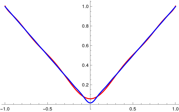
Let’s take f(x) = |x| on [-1,1]. We form its Fourier–Chebyshev series: \[ f(x)\sim \sum _{n=0}^{\infty} a_n\, \omega _n(x),\qquad a_n=\langle f,\omega _n\rangle . \] Because f is even and Tₙ is even for even n, odd for odd n, all odd coefficients 𝑎ₙ vanish: \[ a_{2k+1}=0, \qquad k=0,1,2,\ldots . \] So only even terms remain.

We. compute the coefficients via θ-substitution. Use x = cosθ, θ ∈ [0, π]. Then \[ {\text d}x=-\sin \theta \, {\text d}\theta ,\qquad \sqrt{1-x^2}=\sin \theta ,\qquad \frac{{\text d}x}{\sqrt{1-x^2}} = -{\text d}\theta . \] Also |x| = |cosθ|, and on [0, π], \[ |\cos \theta |=\left\{ \, \begin{array}{ll}\textstyle \cos \theta ,&\textstyle 0\leq \theta \leq \frac{\pi }{2},\\ -\cos \theta ,&\textstyle \frac{\pi }{2}\leq \theta \leq \pi .\end{array}\right. \] For n ≥ 1, \[ a_n = \langle f,\omega _n\rangle =\sqrt{\frac{2}{\pi }}\int _{-1}^1|x|\, T_n(x)\, \frac{{\text d}x}{\sqrt{1-x^2}}=\sqrt{\frac{2}{\pi }}\int _0^{\pi }|\cos \theta |\cos (n\theta )\, {\text d}\theta , \]

For illustration of Theorem 4, we define partial sums \[ S_N(x)=\sum _{n=0}^N a_n\, \omega _n(x). \] We use Mathematica to plot some partial sums.

Theorem 4 (in this Chebyshev setting) says that the corresponding series converges in the mean.

Therefore:

• The Chebyshev–Fourier series of |x| is infinite.
• The partial sums S_N are Chebyshev polynomials (finite combinations of Tₙ).
• These polynomials approximate |x| in the mean square sense with respect to the weight w(x) = 1/√(1-x²).
• The 𝔏²_w-error of approximation goes to zero as N → ∞.

Let’s take f(x) = |x|. This function is even, continuous, and non‑polynomial — perfect for an infinite Chebyshev‑Uₙ expansion.

Compute the Fourier–Chebyshev coefficients: \[ a_n =\langle f,\omega _n\rangle =\sqrt{\frac{2}{\pi }}\int _{-1}^1|x|\, U_n(x)\sqrt{1-x^2}\, {\text d}x. \] Use the substitution x = cosθ,     θ ∈ [0, π]: \[ {\text d}x = -\sin \theta \, {\text d}\theta , \quad \sqrt{1-x^2}=\sin \theta , \quad |x|=|\cos \theta | \] Then \[ a_n = \sqrt{\frac{2}{\pi }}\int _0^{\pi }|\cos \theta |\sin ((n+1)\theta )\sin \theta \, {\text d}\theta . \]

For illustration of Theorem 4, we define the partial sums \[ S_N(x) =\sum _{n=0}^N a_n\, \omega _n(x). \] We use Mathematica to plot some partial sums with 5 and 20 terms.

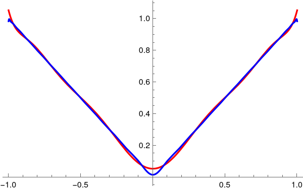
• Each partial sum S_N is a (finite) linear combination of Chebyshev polynomial of the second kind.
• These polynomials approximate |x| in the mean‑square sense with respect to the weight √(1-x²).
• The approximation improves monotonically as N → ∞.
• The infinite series converges in the exact sense guaranteed by Theorem 4.

We present another illustrative example of Theorem 4 using Chebyshev polynomials of the third kind, usually denoted by Vₙ(x). This gives you a genuinely infinite Fourier–Chebyshev expansion in a weighted Hilbert space, exactly parallel to the Uₙ example.

Chebyshev polynomials of the third kind Vₙ form an orthogonal system in the Hilbert space ℌ = 𝔏⊃([−1, 1], w dx) with weight \[ w(x) = (1 - x)^{-1/2} \cdot (1 + x)^{1/2} = \sqrt{\frac{1+x}{1-x}} . \] Chebyshev polynomials of the third kind Vₙ(x) are defined by either the recurrence relation \[ \begin{split} V_{n+1}(x) &= 2x \, V_n(x) - V_{n-1}(x) , \qquad n = 1,2,\ldots , \\ V_0 (x) &= 1 , \quad V_1 (x) = 2x - 1, \end{split} \] or via Chebyshev polynomials of the first and second kind \[ V_n (x) = T_n (x) - \left( 1-x \right) U_{n-1}(x) , \] or through Jacobi polynomials \[ V_n (x) = \frac{n!}{(1/2)_n}\, P_n^{(-1/2, 1/2)}(x) = \frac{P_n^{(-1/2, 1/2)}(x)}{P_n^{(-1/2, 1/2)}(1)} = \frac{4^n \left( n! \right)^2}{(2n)!}\,P_n^{(-1/2, 1/2)}(x) , \] where (1/2)ₙ is the Pochhammer symbol (rising factorial).

Similar to other Chebyshev polynomials, we can express Vₙ as \[ V_{n} (\cos\theta ) = \frac{\cos \left( \frac{2n+1}{2}\,\theta \right)}{\cos \left( \frac{\theta}{2} \right)} . \] Chebyshev polynomials of the third kind are orthogonal on [-1,1] with weight \[ w(x) = (1 - x)^{-1/2} \cdot (1 + x)^{1/2} = \sqrt{\frac{1+x}{1-x}} . \] Then the inner product in ℌ is \[ \langle f,g\rangle =\int_{-1}^1 f(x)\,g(x)\, w(x)\, {\text d}x = \int_{-1}^1 f(x)\,g(x)\, \sqrt{\frac{1+x}{1-x}} \, {\text d}x . \] The orthogonality relation becomes \[ \int _{-1}^1 V_m(x)\,V_n(x)\, w(x)\, {\text d}x =\frac{\pi }{2}\, \delta _{mn}. \] Thus, the corresponding orthonormal system becomes \[ \omega _n(x) =\sqrt{\frac{2}{\pi}}\, V_n(x),\qquad n\geq 0. \] This system is complete in ℌ = 𝔏²([−1,1], wdx), so Theorem 4 applies. The Fourier coefficients are determined as \[ a_n = \langle f, \omega_n \rangle = \sqrt{\frac{2}{\pi}} \int_0^{\pi} f(\cos\theta )\,2\cos\left( \frac{\theta}{2} \right) \cos \left( n + \frac{1}{2} \right) \theta \,{\text d}\theta , \quad n=0,1,2,\ldots . \] For function f(x) = |x|, Mathematica evaliate \[ a_n = \sqrt{\frac{2}{\pi}} \cdot \frac{1}{n \left( n^2 -1 \right) \left( n+2 \right)} \left[ 2n^2 \sin \left( \frac{n\pi}{2} \right) -4n\,\cos \left( \frac{n\pi}{2} \right) -2n^2 \cos \left( \frac{n\pi}{2} \right) -2\,\sin\left( \frac{n\pi}{2} \right) \right] , \quad n\ge 2 . \]

Choose another function with a genuinely infinite expansion: \[ f(x)=\sqrt{1+x}. \] This is a natural choice because:

• it is not a polynomial,
• it is square‑integrable with respect to the weight w(x),
• its Chebyshev–Vₙ expansion is infinite.

Compute the Fourier–Chebyshev coefficients: \[ a_n =\langle f,\omega _n\rangle =\sqrt{\frac{2}{\pi }}\int _{-1}^1 \sqrt{1+x}\, V_n(x)\, w(x)\, {\text d}x. \] Use the substitution x = cosθ,     θ ∈ [0, π]. Then: \[ V_n (\cos \theta ) = \frac{\cos (n + 1/2)\theta )}{\cos ( \theta/2 )} , \quad n=0,1,2,\ldots , \] and \[ {\text d}x = -\sin \theta \, {\text d}\theta , \qquad \sqrt{1-x} = \sqrt{2}\,\sin (\theta /2) . \] Putting everything together, we get \[ a_n = \sqrt{\frac{2}{\pi }}\int_{0}^{\pi} \frac{1+\cos\theta}{\sqrt{1-\cos\theta}} \, \frac{\cos (n + 1/2)\theta )}{\cos ( \theta/2 )}\,\sin\theta\,{\text d}\theta , \]

• Each S_N is a finite Chebyshev polynomial of the third kind.
• These polynomials approximate \sqrt{1+x} in the mean‑square sense with respect to the weight w(x)=1/(\sqrt{1-x^2}(1+x)).
• The approximation improves monotonically as N → ∞.
• The infinite series converges exactly as Theorem 4 guarantees.

It is a dense family in ℌ where Parseval's identity holds. Let us consider the set \[ \mathcal{D} = \left\{ f\in 𝔏^2(\mathbb{R}):f\mathrm{\ has\ compact\ support\ and\ is\ piecewise\ constant\ on\ dyadic\ intervals\ }[m2^{-N},(m+1)2^{-N})\right\} . \] These dyadic step functions are dense in 𝔏²(ℝ) (they approximate any 𝔏² function by local averaging on fine dyadic grids).

Wavelet expansion on \( \displaystyle \quad \mathcal{D}\ : \ \) For such an f, only finitely many Haar coefficients \[ c_{j,k}=\langle f,\psi _{j,k}\rangle \] are nonzero, because f is constant on sufficiently fine dyadic intervals and has compact support.

Parseval's identity on \( \displaystyle \quad \mathcal{D}: \ \) For each \( \displaystyle \quad f\in \mathcal{D}, \) \[ \| f\| _{𝔏^2(\mathbb{R})}^2=\sum _{j,k}|\langle f,\psi _{j,k}\rangle |^2, \] where the sum is actually finite (so there is no convergence issue). Thus Parseval’s identity holds for all f in the dense set \( \displaystyle \quad \mathcal{D}. \)

Theorem 6 says: An orthonormal system { ωₙ } in ℌ is closed (complete) if and only if Parseval’s identity holds for a dense family of functions.

We have: { ψ_j,k } is orthonormal in 𝔏²(ℝ). There is a dense set \( \displaystyle \quad \mathcal{D} \subset 𝔏^2(\mathbb{R}) \) (dyadic step functions) such that Parseval's identity holds for every \( \displaystyle \quad f\in \mathcal{D}. \) Therefore, by Theorem 6, the Haar wavelet system { ψ_j,k } is closed, i.e., complete in 𝔏²(ℝ). We have:

• { ψ_j,k } is orthonormal in 𝔏²(ℝ).
• There is a dense set \( \displaystyle \quad \mathcal{D} \subset 𝔏^2;(\mathbb{R}) \) (dyadic step functions) such that Parseval holds for every f ∈ \( \displaystyle \quad \mathcal{D}. \)

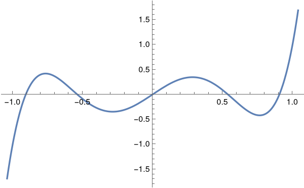
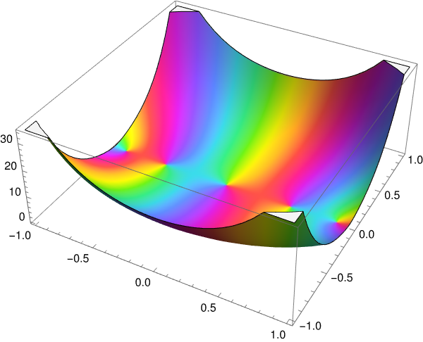
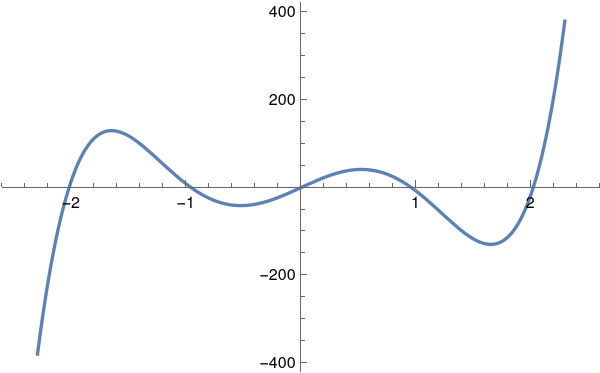
With the aid of Mathematica, we plot Legendre's polynomial P₅ for real and complex argument.

We use the Gram-Schmidt orthogonalization procedure to generate Legendre polynomials from the list of monomials \[ 1 , \ x, \ x^2 , \ x^3 , \ \ldots , x^n , \ \ldots , \] in Hilbert space ℌ = 𝔏²([−1,1]) with inner product \[ \langle f \mid g \rangle = \int_{-1}^1 f(x)\,g(x)\,{\text d} x. \]

The first two items, ϕ₀ = 1 and ϕ₁ = x, in the list { xⁿ } are orthogonal: \[ \langle \phi_0 \mid \phi_1 \rangle = \langle 1 \mid x \rangle = \int_{-1}^1 x\,{\text d} x = 0 . \] So we can set ψ₀ = ϕ₀ = 1 and ψ₁ = ϕ₁ = x. The next element in the orthogonal list is taken as a linear combination \[ \psi_2 = \phi_2 + b_{20}\psi_0 + b_1\psi_1 = x^2 + b_{20} + b_{21} x . \] This vector ψ₂ must be orthogonal to both, ψ₀ and ψ₁. So this leads to \begin{align*} 0&= \langle \psi_2 \mid \phi_0 \rangle = \langle x^2 \mid 1 \rangle + b_{20} \langle 1 \mid 1 \rangle + b_{21} \langle x \mid 1 \rangle = \frac{2}{3} + 2\,b_{20} , \\ 0&= \langle \psi_2 \mid \phi_1 \rangle = \langle x^2 \mid x \rangle + b_{20} \langle 1 \mid x \rangle + b_{21} \langle x \mid x \rangle = b_{21}\,\frac{2}{3} . \end{align*}

Since our algorithm of the Gram–Schmidt version keeps the leading coefficient 1, then each qₙ(x) is monic: \[ q_n(x) = x^n + \mathrm{(lower\ degree\ terms)}. \] By construction:

• degree of qₙ(x) = n,
• ⟨ qₙ∣qₖ ⟩ = 0 for n ≠ k,
• and the leading coefficient of qₙ is 1.

Fix n. Consider all polynomials of degree at most n. Among them, look at monic degree-n polynomials: \[ p(x) = x^n + a_{n-1} x^{n-1} + \dots + a_0 . \] The orthogonality conditions \[ \langle p \mid x^k \rangle = 0,\quad k=0,1,\dots ,n-1 \] are n linear equations in the n unknowns 𝑎₀, 𝑎₁, … , 𝑎_n-1. The Gram–Schmidt construction shows that this system has a solution (namely, the coefficients of qₙ are determined). Because the inner product is nondegenerate on polynomials, this system has a unique solution. Hence:

Legendre polynomials satisfy the same orthogonality conditions, \[ \langle P_n \mid P_k \rangle = \int_{-1}^1 P_n (x)\, P_k (x)\,{\text d}x = 0 \quad\mbox{for}\quad n \ne k . \] For k < n, we integrate by parts \begin{align*} A_{kn} &= \langle x^k \mid P_n \rangle = \int_{-1}^1 x^k P_n (x)\,{\text d}x \\ &= \frac{1}{2^n n!} \int_{-1}^1 x^k \left[ \left( x^2 -1 \right)^n \right]^{(n)} {\text d}x \\ &= \left. \frac{x^k}{2^n n!} \,\frac{{\text d}^{n-1}}{{\text d}x^{n-1}} \left( x^2 -1 \right)^n \right\vert_{x=-1}^{x=1} - \frac{k}{2^n n!} \int_{-1}^1 x^{k-1}\left[ \left( x^2 -1 \right)^n \right]^{(n-1)} {\text d}x \tag{9.3} \end{align*} Since polynomial (x² − 1)ⁿ has zeroes of multiplicity n at points ±1, all its derivatives up to the order n−1 vanish at these points. Hence, all terms outside integral in Eq.(9.3) are zero. Then we integrate k−1 times by parts integral (9.3) and obtain for k < n that \begin{align*} A_{kn} &= \frac{(-1)^k k!}{2^n n!} \int_{-1}^1 \left[ \left( x^2 -1 \right)^n \right]^{(n-k)} {\text d}x \\ &= \left. \frac{(-1)^k k!}{2^n n!} \,\frac{{\text d}^{n-k-1}}{{\text d}x^{n-k-1}} \left( x^2 -1 \right)^n \right\vert_{x=-1}^{x=1} = 0 . \end{align*} So Legendre's polynomials are orthogonal.

The leading coefficient of the classical Legendre polynomial (9.1) is \[ \frac{(2n)^{\underline{n}}}{2^n n!} = \frac{2n \left( 2n-1 \right) \cdots \left( n+1 \right)}{2^n n!} = \frac{(2n)!}{2^n \left( n! \right)^2} . \] Therefore, if we divide by this coefficient the Legendre polynomial, we obtain a monic polynomial: \[ \tilde{P}_n (x) = \frac{2^n \left( n! \right)^2}{(2n)!}\, P_n (x) = \frac{n!}{(2n)!}\,\frac{{\text d}^n}{{\text d}x^n} \left( x^2 -1 \right)^n . \]

Let us calculate their norms: \begin{align*} \| P_n \|^2 &= \int_{-1}^1 P_n^2 (x)\,{\text d} x = \frac{(2n)!}{2^n \left( n! \right)^2} \int_{-1}^1 x^n P_n (x)\,{\text d} x \\ &= \frac{(2n)!}{2^{2n} \left( n! \right)^2} \int_{-1}^1 x^n \left[ \left( x^2 -1 \right)^n \right]^{(n)} {\text d} x \\ &= (-1)^n \frac{(2n)!}{2^{2n} \left( n! \right)^2} \int_{-1}^1 \left( x^2 -1 \right)^n {\text d} x . \end{align*} The latter integral we also evaluate by integrating by parts. \begin{align*} (-1)^n \frac{(2n)!}{2^{2n} \left( n! \right)^2} \,\| P_n \|^2 &= \int_{-1}^1 \left( x+1 \right)^n \left( x-1 \right)^n {\text d} x \\ &= \left. \left( x+1 \right)^n \left( x-1 \right)^{n+1} \frac{1}{n+1} \right\vert_{x=-1}^{x=1} - \frac{n}{n+1} \int_{-1}^1 \left( x+1 \right)^{n-1} \left( x-1 \right)^{n+1} {\text d} x \\ &= (-1)^n \,\frac{\left( n! \right)^2}{(2n)!} \int_{-1}^1 \left( x-1 \right)^{2n} {\text d} x \\ &= (-1)^n \,\frac{\left( n! \right)^2}{(2n)!} \,\frac{2^{2n+1}}{2n+1} . \end{align*} Finally, we get \[ ,\| P_n \|^2 = \int_{-1}^1 P_n^2 (x) \,{\text d}x = \frac{2}{2n+1} . \]

We summarize some facts regarding the (classical) Legendre polynomials Pₙ that are defined by Rodrigues’ formula (9.1).

• Degree of Pₙ = n.
• Orthogonality: \[ \int _{-1}^1 P_n(x)P_m(x)\, dx=0,\quad n\neq m. \] In particular, for fixed n, Pₙ is orthogonal to every polynomial of degree less than n.
• Leading coefficient: Pₙ has leading term \[ P_n(x)=\frac{2^n}{(2n)!}\, (2n-1)!!\, x^n + \cdots , \] so the leading coefficient is nonzero.

• \( \displaystyle \ \tilde {P}_n \ \) is monic,
• Degree of monic polynomial \( \displaystyle \ \tilde {P}_n \ \) is n,
• \( \displaystyle \ \tilde {P}_n \ \) is orthogonal to all polynomials of degree less than n.

The Laguerre polynomials, named after the French mathematician Edmond Laguerre (1834–1886), may be defined by the Rodrigues formula, \[ L_n (x) = \frac{e^x}{n!}\,\frac{{\text d}^n}{{\text d} x^n} \left( e^{-x} x^n \right) = \frac{1}{n!} \left( \frac{\text d}{{\text d}x} -1 \right)^n x^n , \quad n=0,1,2,\ldots . \tag{10.1} \] Actually, there is no evidence that Edmond Laguerre worked or was familiar with the Laguaerre polynomials that were invented by Pafnuty Chebyshev in 1859, \[ L_n (x) = \sum_{k=0}^n \frac{(-1)^k}{k!} \,\binom{n}{k} \,x^k , \tag{10.2} \] where \( \displaystyle \ \binom{n}{k} = \frac{n!}{k!\,(n-k)!} \ \) is the binomial coefficient.

An orthogonalization procedure is applied to a given linearly independent sequence { ϕ₀, ϕ₁, … , ϕₙ, …} to define \begin{align*} u_0 &= \phi_0 , \\ u_n &= \phi_n - \sum_{k=0}^{n-1} \frac{\langle \phi_n \mid u_k \rangle}{\langle u_k \mid u_k \rangle}\, \phi_k , \quad n\ge 1. \end{align*} Then { uₙ } is an orthogonal sequence, and each uₙ lies in span{ ϕ₀, ϕ₁, … , ϕₙ }.

If we want monic polynomials, we simply normalize each uₙ by dividing by its leading coefficient: \[ p_n(x)\; =\; \frac{1}{\mathrm{(leading\ coefficient\ of\ }u_n)}\, u_n(x). \] Then:

• Each pₙ is a polynomial of degree n.
• Each pₙ is monic.
• The family { pₙ }_n≥0 is orthogonal with respect to ⟨ · ∣ · ⟩.

The key idea now is: Laguerre polynomials also form such a sequence. If we show that the (appropriately normalized) Laguerre polynomials are monic and orthogonal with respect to the same inner product, then a uniqueness argument will force { pₙ } to coincide with them.

The Laguerre polynomials satisfy the orthogonality relation \[ \langle L_n \mid L_m \rangle = \int _0^{\infty }L_n(x)\, L_m(x)\, e^{-x}\, {\text d}x = \begin{cases} 0, &\quad n\neq m , \\ 1 , &\quad n=m . \end{cases} \] Mathematica confirms:

1. \( \displaystyle \ \hat {L}_n(x) \ \) is monic of degree n.
2. List of monic polynomials \( \displaystyle \ \{ \hat {L}_n\} \) is orthogonal with respect to \( \displaystyle \ \langle f,g\rangle =\int _0^{\infty }f(x)g(x)e^{-x}\, {\text d}x.\)
3. Once that is done, uniqueness of monic orthogonal polynomials will give \( \displaystyle \ \hat {L}_n = p_n \ \) for all n.

We now show that { Lₙ } (and hence \( \displaystyle \ \{ \hat {L}_n\} \) ) is orthogonal with respect to \( \displaystyle \ \langle f,g\rangle =\int _0^{\infty }f(x)g(x)e^{-x}\, {\text d}x. \ \) Take m < n. Consider \[ \int _0^{\infty }L_n(x)\, x^m\, e^{-x}\, {\text d}x. \] Using the Rodrigues formula, we get \[ \int _0^{\infty} x^m\, \frac{e^x}{n!}\,\frac{{\text d}^n}{{\text d} x^n} \left( e^{-x} x^n \right) e^{-x}\, {\text d}x = \int _0^{\infty} x^m\, \frac{1}{n!}\,\frac{{\text d}^n}{{\text d} x^n} \left( e^{-x} x^n \right) {\text d}x . \] Integrate by parts n times. Each integration by parts moves one derivative from \( \displaystyle \ \frac{{\text d}^n}{{\text d}x^n}(e^{-x}x^n) \ \) onto x^m. Because m < n, after m + 1 derivatives of x^m becomes zero. More systematically:

• After k integrations by parts, the integrand involves \( \displaystyle \ \frac{{\text d}^{n-k}}{{\text d}x^{n-k}}(e^{-x}x^n) \times \frac{d^k}{dx^k}x^m. \)
• For k>m, \( \displaystyle \ \frac{{\text d}^k}{{\text d}x^k}x^m=0. \)

Uniqueness of monic orthogonal polynomials follows from a simple but powerful uniqueness lemma.

On the other hand, \[ 0 = \langle p_n,r_n\rangle =\langle p_n,p_n-q_n\rangle =\langle p_n,p_n\rangle -\langle p_n,q_n\rangle . \] But qₙ is also orthogonal to all polynomials of degree < n, and pₙ has degree n, so the only way ⟨ pₙ , qₙ ⟩ can be nonzero if pₙ and qₙ are linearly dependent. However, they are both monic of the same degree, so if they are linearly dependent, each of them must be a scalar multiple of another. This scalar must be 1, i,e,, qₙ ≡ pₙ. In that case, rₙ = 0 and we done.

A more direct argument: since rₙ has degree ≤ n-1, orthogonality of pₙ and qₙ to all polynomials of degree ≤ n-1 implies \[ \langle p_n, r_n\rangle = \langle q_n, r_n\rangle = 0. \] Since rₙ = pₙ − qₙ has degree ≤ n-1, we also get \[ \langle q_n,r_n\rangle =0\; \Rightarrow \; \langle q_n,p_n\rangle =\langle q_n,q_n\rangle . \] But \( \displaystyle \ \langle p_n,q_n\rangle =\langle q_n,p_n\rangle , \ \) so \[ \langle p_n,p_n\rangle =\langle q_n,q_n\rangle . \] Then \[ 0=\langle p_n,r_n\rangle =\langle p_n,p_n\rangle -\langle p_n,q_n\rangle =\langle p_n,p_n\rangle -\langle q_n,q_n\rangle =0, \] which is consistent but doesn’t yet force equality. To pin it down, note that if rₙ ≠ 0, then rₙ has degree ≤ n-1 and is nonzero, so it cannot be orthogonal to all polynomials of degree ≤ n-1 unless the inner product is degenerate. Since our inner product is nondegenerate on polynomials (because \( \displaystyle \ \int _0^{\infty }|p(x)|^2e^{-x}dx=0 \ \) implies p ≡ 0), we must have rₙ = 0. Hence, pₙ = qₙ.

In short: for a nondegenerate inner product, there is at most one monic orthogonal polynomial of each degree.     ▣

This gives us a conclusion: the Gram–Schmidt process gives the Laguerre polynomials.

Application of the Gram–Schmidt process to the sequence of monomials { 1, x, x², … , xⁿ, …} produces a sequence of monic orthogonal polynomials { pₙ(x) }_n≥0, where \[ p_n(x)=x^n+\mathrm{(lower\ degree\ terms)},\quad \deg p_n=n, \] and \[ \langle p_n,p_m\rangle =0\quad \mathrm{for\ }n\neq m. \] These pₙ(x) will turn out to satisfy a three-term recurrence (usually called the difference equation): \[ x\, p_n(x)\; =\; p_{n+1}(x)+\alpha _n\, p_n(x)+\beta _n\, p_{n-1}(x),\qquad n\geq 1, \] with \[ p_0 (x) = 1,\qquad p_1(x) =x-\alpha _0, \] and real coefficients αₙ, βₙ > 0. The reason is purely Gram–Schmidt/linear algebra:

• Degree constraint: x pₖ has degree n+1, so it can be expressed in the basis { p₀, p₁, … , p_n+1 }.
• Monicity: both x pₖ and p_n+1 are monic of degree n+1, so the coefficient in front of p_n+1 must be 1.
• Orthogonality: the component of x pₙ along pₖ for k ≤ n-2 must vanish, because \[ \langle xp_n, p_k\rangle =\langle p_n, xp_k\rangle , \]
• and x pₖ is a linear combination of p₀, p₁, … , p_k+1, all orthogonal to pₙ when k+1 ≤ n-1. So ⟨ x pₖ∣pₖ ⟩ = 0 if |n-k|>1. Hence, only p_n+1, pₖ, p_n-1 can appear in the recurrence.

Now use orthogonality, and take inner product with p_j: \[ \left\langle x\,p_n \mid p_j \right\rangle = \left\langle p_{n+1} \mid p_j \right\rangle + \sum _{k=0}^n a_{n,k}\left\langle p_k,p_j\right\rangle . \] Moreover, the coefficients are given directly by inner products: \[ \alpha_n =\frac{\langle xp_n , p_n\rangle }{\langle p_n , p_n\rangle },\qquad \beta _n =\frac{\langle xp_n , p_{n-1}\rangle }{\langle p_{n-1} , p_{n-1}\rangle }. \]

In our case, we know that pₙ = (−1)ⁿn! Lₙ, so \[ \langle p_n , p_n\rangle = \| p_n \|^2 = \left( n! \right)^2 \int_0^{\infty} L_n^2 (x)\,e^{-x} {\text d} x = \left( n! \right)^2 . \] Since \[ x\,L_n (x) = \left( 2n+1 \right) L_n (x) - \left( n+1 \right) L_{n+1} (x) -n\,L_{n-1} (x) , \] we find \[ \langle xp_n \mid p_n\rangle = \left( 2n+1 \right) \| p_n \|^2 = \left( 2n+1 \right) \left( n! \right)^2 . \] This gives \[ \alpha_n = 2n+1 , \qquad \beta_n = -n . \]    ■

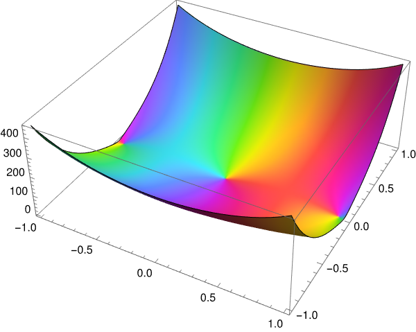
Hermite polynomials, denoted by Hₙ(x), can be defined recursively \[ H_{n+1} (x) = 2x\,H_n (x) - 2n\,H_{n-1} (x) , \qquad H_0 (x) = 1, \quad H_1 (x) = 2x. \tag{11.1} \] Mathematica has a build-in command:

Be aware that there are the "probabilist's Hermite polynomials", given by \[ \mbox{He}_n ( x ) = ( − 1 )^n e^{x^2 /2} \frac{{\text d}^n}{{\text d} x^n}\, e^{− x^2 /2} , \qquad n=0,1,2,\ldots . \]

The "physicist's Hermite polynomial" Hₙ(x) can be derived by orthogonalization from the list of monomials \[ \phi_n (x) = x^n \qquad \left( n=0,1,2,\ldots \right) , \] in Hilbert space ℌ = 𝔏²(ℝ, wdx) = 𝔏^²_w with the weight function \[ w(x) = e^{-x^2} . \] These monomials { xⁿ } are linearly independent, but not orthogonal in ℌ. We verify their linearly independence with Mathematica by showing that their Wronskian is not zero.

Starting with n = 0, let \[ \psi_0 = \phi_0 = 1 , \quad \omega_0 = \frac{1}{\| 1 \|} = \frac{1}{\pi^{1/4}} = \pi^{-1/4} \] because \[ \int_{-\infty}^{\infty} {\text d} x = \sqrt{\pi} . \]

For n = 2, let \[ \psi_2 = \phi_2 + b_{20}\phi_0 + b_{21} \phi_1 = x^2 + b_{20} + b_{21} x . \] Its inner product with ϕ₀ = 1 gives \[ 0 = \langle \psi_2 \mid 1 \rangle = \int_{-\infty}^{\infty} \left( x^2 + b_{20} + b_{21} x \right) e^{-x^2} {\text d} x = b_{20} \sqrt{\pi} + \frac{\sqrt{\pi}}{2} . \]

For n = 3, let \[ \psi_3 = \phi_3 + b_{30}\phi_0 + b_{31} \phi_1 +b_{32} \phi_2 = x^3 + b_{32} x^2 + b_{31} x + b_{30} . \] Taking the inner product with 1, we get \[ 0 = \langle \psi_3 \mid 1 \rangle = b_{30} \| 1 \|^2 + b_{32} \langle x^2 \mid 1 \rangle = \sqrt{\pi} \left( b_{30} + \frac{b_{32}}{2} \right) . \] Similarly, we have \begin{align*} 0 &= \langle \psi_3 \mid x \rangle = b_{31} \langle x \mid x \rangle + \langle x^3 \mid x \rangle = \sqrt{\pi} \left( \frac{1}{2}\,b_{31} + \frac{3}{4} \right) , \\ 0 &= \langle \psi_3 \mid x^2 \rangle = b_{32} \langle x^2 \mid x^2 \rangle + b_{30} \langle 1 \mid x^2 \rangle = \sqrt{\pi} \left( b_{32}\,\frac{3}{4} + b_{30}\,\frac{1}{2} \right) . \end{align*} Therefore, ψ₃ = x³ − 3/2 = 8 H₃(x). So empirically, we have \[ \psi_n (x) = 2^n H_n (x) = \left( -2 \right)^n e^{x^2} \frac{{\text d}^n}{{\text d} x^n} \left( e^{-x^2} \right) , \quad n = 0,1,2,\ldots . \tag{11.2} \] This system of functions { ψₙ(x) } is orthogonal by construction. We are going to prove that the Gram--Schmidt process defines (up to a non-zero multiple) the "physicists" Hermite polynomials Hₙ(x) in two ways. First, we show that the orthogonalization leads to recurrence (11.1); then we rederive the Rodrigues formula for the n-th Hermite polynomial Hₙ(x).

We are going to derive a three‑term recurrence from Gram–Schmidt orthogonalization procedure. A key structural fact: for any orthogonal polynomial system { pₙ } with respect to a positive weight on an interval, multiplication by x acts tridiagonally: \[ x\,p_n (x) = a_{n+1} p_{n+1}(x) + b_n p_n(x) + a_n p_{n-1}(x), \] with suitable coefficients 𝑎ₙ, bₙ.

Here, because the weight \( \displaystyle \ e^{-x^2} \ \) is even and pₙ has parity (-1)ⁿ, we get bₙ = 0 (the integrals defining bₙ vanish by parity). So we expect \[ x\,p_n(x) = a_{n+1}p_{n+1}(x) + a_n p_{n-1}(x). \] To compute the coefficients, we take inner products with p_n+1 and p_n-1. \[ \langle xp_n,p_{n+1}\rangle =a_{n+1}\langle p_{n+1},p_{n+1}\rangle , \] so we determine coefficient 𝑎_n+1: \[ a_{n+1}=\frac{\langle xp_n,p_{n+1}\rangle }{\| p_{n+1}\| ^2}. \] Coefficient 𝑎ₙ: \[ \langle x\,p_n \mid p_{n-1}\rangle = a_n\langle p_{n-1} \mid p_{n-1}\rangle . \] Hence, \[ a_n=\frac{\langle xp_n,p_{n-1}\rangle }{\| p_{n-1}\| ^2}. \] Because pₙ is monic (leading coefficient is 1), the leading term of x pₙ is xⁿ⁺¹, and the leading term of p_n+1 is also xⁿ⁺¹. This forces \[ a_{n+1}=1. \] Thus, the recurrence simplifies to \[ x\,p_n(x) = p_{n+1}(x) + a_n p_{n-1}(x). \] We can determine 𝑎ₙ by comparing norms or by direct integration. A standard computation (or comparison with the known Hermite recurrence) gives \[ a_n = \frac{n}{2}. \] So the Gram–Schmidt polynomials satisfy \[ p_{n+1}(x) = x\,p_n(x)-\frac{n}{2}p_{n-1}(x), \] with \[ p_0(x)=1,\quad p_1(x)=x. \] Multiplying by 2ⁿ, define \[ H_n (x) = 2^n p_n(x). \] Then \[ H_{n+1}(x) = 2x\,H_n(x)-2n\,H_{n-1}(x), \] which is exactly the standard Hermite recurrence (11.1). So the three‑term recurrence is inherited from Gram–Schmidt process.

Next we prove that Gram–Schmidt polynomials are exactly Hermite polynomials up to some numerical multiple. We start by deriving the Rodrigues' formula. Let us evaluate derivatives of the weight function: \begin{align*} u &= e^{-x^2} , \\ u' &= -2x\,e^{-x^2} , \\ u'' &= \left( 4x^2 -2 \right) e^{-x^2} , \\ u''' &= - \left( 8x^3 -12\,x \right) e^{-x^2} , \\ \vdots & \qquad \vdots \\ u^{(n)} &= (-1)^n H_n (x)\, e^{-x^2} , \end{align*} where Hₙ(x) is the Hermite polynomial. From the above, we have \[ H_n (x) = (-1)^n u^{(n)} (x) = (-1)^n e^{x^2} \frac{{\text d}^n}{{\text d} x^n} \, e^{-x^2} , \quad n=0,1,2,\ldots . \] This polynomial is of degree n and its leading coefficient is 2ⁿ.

We prove it by induction. For n = 0 and n = 1, the statement is true. Suppose that it is valid up to n, that is, the polynomial Hₙ(x) is of degree n and its leading coefficient is 2ⁿ. We determine the Hermite polynomial of order n+1: \begin{align*} u^{(n+1)} &= (-1)^n e^{-x^2} \frac{\text d}{{\text d}x}\, H_n (x) -2x \left( -1 \right)^n H_n (x)\, e^{-x^2} \\ &= (-1)^{n+1} 2x\,H_n (x)\, e^{-x^2} + (-1)^n e^{-x^2} \frac{\text d}{{\text d}x}\, H_n (x) . \end{align*} The first multiple 2x Hₙ(x) is a polynomial of degree n+1 and its leading term is 2ⁿ⁺¹ because Hₙ is of degree n and has leading coefficient 2ⁿ by assumption. The second term is a polynomial of degree n−1, so it does not contribute to the leading term.

Let us introduce the function \[ \psi_n (x) = H_n (x)\, e^{-x^2 /2} . \] For any n, function ψₙ is square integrable, so the system { ψₙ }_n≥0 is orthogonal in 𝔏²(ℝ). Indeed, integration by parts yields \begin{align*} \langle u^{(n)} \mid v \rangle &= \int_{-\infty}^{\infty} u^{(n)} (x)\,v(x)\,{\text d}x \\ &= \left[ u^{(n-1)}(x)\,v(x) - u^{(n-2)}(x)\,v'(x) + \cdots + (-1)^{n-1} u(x)\, v^{(n-1)} (x) \right]_{-\infty}^{\infty} \\ & \quad +(-1)^n \int_{\mathbb{R}} u(x)\,v^{(n)} {\text d}x . \tag{11.3} \end{align*} Assuming n > k, we calculate \begin{align*} \langle \psi_n \mid \psi_k \rangle &= \int_{-\infty}^{\infty} H_n (x)\,H_k (x)\, e^{-x^2} {\text d}x \\ &= (-1)^n \int_{\mathbb{R}} u^{(n)} (x) \,H_k (x)\,{\text d}x . \end{align*} Applying integration by parts formula (11.3), we get \begin{align*} \langle \psi_n \mid \psi_k \rangle &= (-1)^n \int_{\mathbb{R}} u^{(n)} (x) \,H_k (x)\,{\text d}x \\ &= (-1)^{2n} \int_{\mathbb{R} u(x)\, H_k^{(n)} \,{\text d} x = 0 \end{align*} because Hₖ(x) is a polynomial of degree k < n.    ■

1. Byron, F.W. and Fuller, R.W., Mathematics of Classical and Quantum Physics, Dover Publications, 1992.
3. I. Todhunter, An Elementary Treatise on Laplace's, Lamé's, and Bessel's Functions, MacMillan, 1875 (London).