Return to computing page for the first course APMA0330
Return to computing page for the second course APMA0340
Return to computing page for the fourth course APMA0360
Return to Mathematica tutorial for the first course APMA0330
Return to Mathematica tutorial for the second course APMA0340
Return to Mathematica tutorial for the fourth course APMA0360
Return to the main page for the course APMA0330
Return to the main page for the course APMA0340
Return to the main page for the course APMA0360
Introduction to Linear Algebra with Mathematica
Glossary
Laplace equation in polar coordinates
Polar coordinates locate a point in a plane ℝ² using a distance (r) from a central point (the "pole") and an angle (θ) from a reference ray (the "polar axis"). These two variables (r, θ) have different dimensional units in opposite to Cartesian coordinates (x, y), which use two distances along perpendicular axes. The angular coordinate is usually denoted by φ, θ, or t. The angular coordinate is specified as φ by ISO standard 31-11, now 80000-2:2019. However, in mathematical literature the angle is often denoted by θ instead.
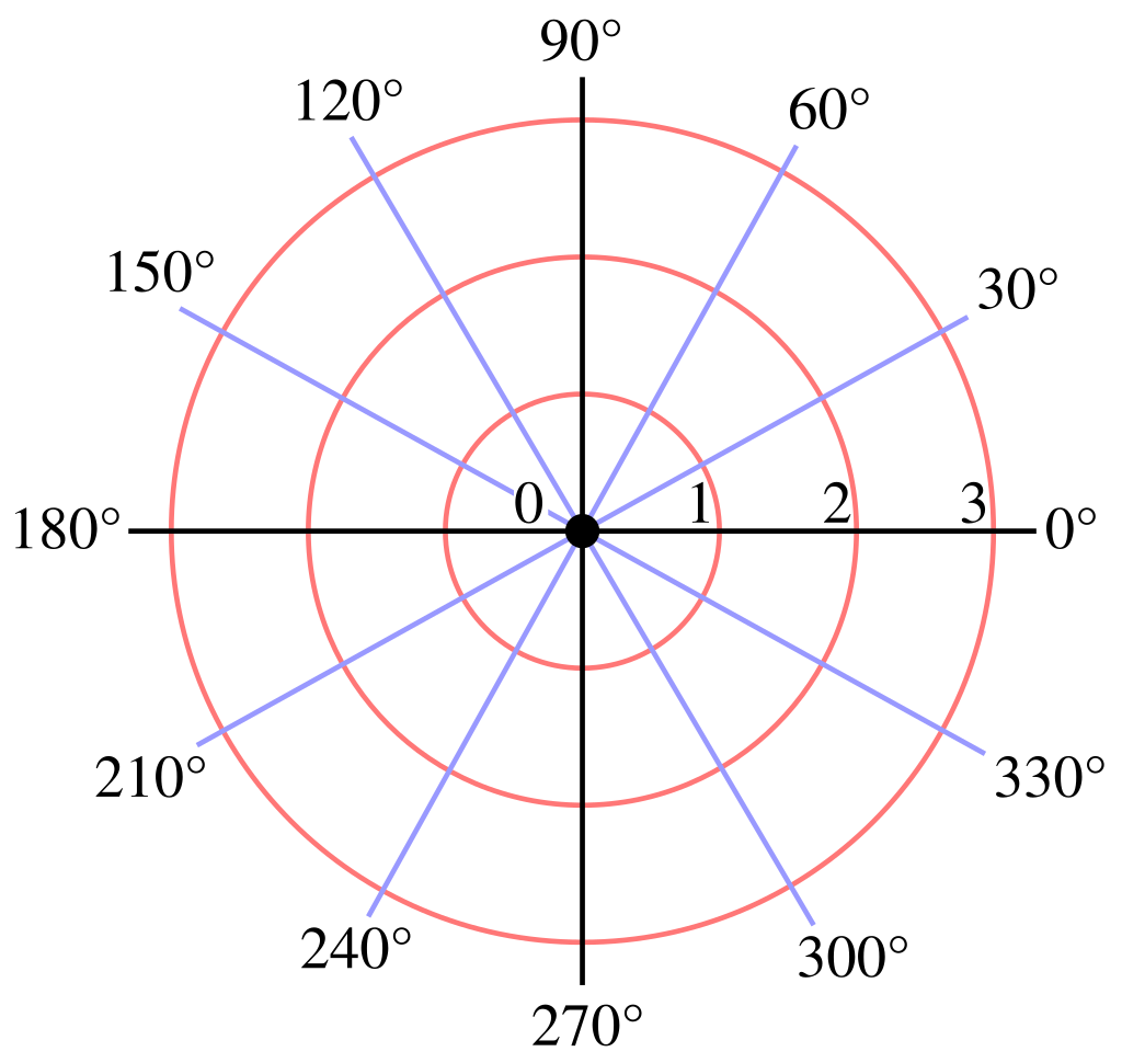
In polar coordinates, the angle (θ) is the measure of the angle from a reference direction (the polar axis, typically the positive x-axis) to the line segment connecting the origin to a point. This angle is measured in a counterclockwise direction, and it, along with the radial distance (r), defines the position of the poin. The pole (origin) itself has no polar coordinates---it is a singular point in this coordinates.
The Laplace equation in polar coordinates (r, θ) can be written as
To solve this boundary value problem, we employ the method of separation of variables. Namely, we seek partial nontrivial solutions of the Laplace equation (written in polar coordinates) \[ \nabla^2 \phi = \frac{1}{r} \frac{\partial}{\partial r} \left( r \frac{\partial \phi}{\partial r} \right) + \frac{1}{r^2} \frac{\partial^2 \phi}{\partial \theta^2} = 0 \] that are represented in product form ϕ(r, θ) = R(r) Θ(θ), where R(r) is a function of radial variable and Θ(θ) is a function of angle variable only. Substituting this product into Laplace's equation, we get \[ \frac{1}{r}\,\frac{\text d}{{\text d}r} \left( r\,\frac{{\text d}R(r)}{{\text d}r} \right) \Theta (\theta ) + \frac{R(r)}{r^2}\, \frac{{\text d}^2 \Theta}{{\text d}\theta^2} = 0 , \] which leads to separation of variables (upon multiplication by r² and division by ϕ(r, θ)): \[ \frac{r}{R(r)}\, \frac{\text d}{{\text d}r} \left( r\,\frac{{\text d}R(r)}{{\text d}r} \right) = - \frac{1}{\Theta (\theta )}\,\frac{{\text d}^2 \Theta}{{\text d}\theta^2} = \lambda . \] So we get two ordinary differential equations with unknown yet parameter λ, \[ r^2 R'' + r\, R' - \lambda\,R = 0 , \qquad \Theta'' + \lambda\,\Theta = 0 . \] Since Θ(θ) must be periodic function of period 2π, we obtain the Sturm--Liouville (S.-L. for short) problem: \[ \begin{cases} \Theta'' + \lambda\,\Theta = 0 , \\ \Theta (\theta ) = \Theta (\theta + 2\pi ) . \end{cases} \] To solve this Sturm--Liouville problem, we need to consider three cases whether λ is negative, equals to zero, or positive. If λ is negative, the general solution of differential equation Θ′′ + λΘ = 0 is \[ \Theta (\theta ) = c_1 e^{\theta\sqrt{-\lambda}} + c_2 e^{-\theta\sqrt{-\lambda}} , \] with some real constants c₁ and c₂. This exponential function cannot be periodic, so we reject this case and claim that the given S,-L, problem has no eigenvalues for negative λ,
When λ = 0, the differential equation Θ′′ = 0 has the general solution \[ \Theta (\theta ) = c_1 + c_2 \theta . \] Since the linear term cannot be periodic, we have to set c₂ = 0; so λ = 0 is an eigenvalue to which corresponds the eigenfunction Θ(θ) = constant.
When λ is a positive number, the general solution of the differential equation Θ′′ + λΘ = 0 is \[ \Theta (\theta ) = c_1 \cos \left( \theta\sqrt{\lambda} \right) + c_2 \sin \left( \theta\sqrt{\lambda} \right) , \] with some real constants c₁ and c₂. This trigonometric function can be periodic with period 2π if and only if λ = n² is a square of a positive integer (why positive, see the previous example). So the solution of this S.-L. problem gives eigenvalues and eigenfunctions: \[ \lambda_n = n^2 , \quad \Theta_n = a_n \cos n\theta + b_n \sin n\theta ,\qquad n=0,1,2,\ldots . \] Substitution of this λ = n² into R-equation yields the Euler ODE \[ r^2 R'' + r\, R' - n^2\,R = 0 , \qquad n= 0,1,2,\ldots . \] We start with n = 0, which is reduced to \[ r^2 R'' + r\, R' = 0 \qquad \iff \qquad r\,\frac{\text d}{{\text d}r} \left( r\,\frac{{\text d}R}{{\text d}r} \right) = 0 . \] This differential equation has two linearly independent solutions R = constant and R = lnr. We reject the latter because logarithm function is unbounded at infinity (the regularity condition requires all functions to be bounded). So we get one function R₀(r) = constant corresponding to eigenvalue λ = 0.
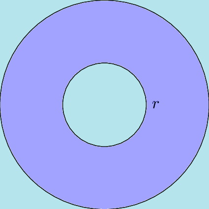
We can also solve this problem using the conformal mapping w = f(z) = 1/z. This function maps points in the z-plane, (x, y), to points in the w-plane, (u, v), by f(x + ⅉy) = (u + ⅉv), where ⅉ (also is denoted by j) is the imaginary unit on the complex plane so ⅉ² = −1. This mapping maps the interior of the unit circle to the exterior of the unit circle in the w-plane.
To solve this boundary value problem, we employ the method of separation of variables. Namely, we seek partial nontrivial solutions of the Laplace equation (written in polar coordinates) \[ \nabla^2 \phi = \frac{1}{r} \frac{\partial}{\partial r} \left( r \frac{\partial \phi}{\partial r} \right) + \frac{1}{r^2} \frac{\partial^2 \phi}{\partial \theta^2} = 0 \] that are represented in product form ϕ(r, θ) = R(r) Θ(θ), where R(r) is a function of radial variable and Θ(θ) is a function of angle variable only. Substituting this product into Laplace's equation, we get \[ \frac{1}{r}\,\frac{\text d}{{\text d}r} \left( r\,\frac{{\text d}R(r)}{{\text d}r} \right) \Theta (\theta ) + \frac{R(r)}{r^2}\, \frac{{\text d}^2 \Theta}{{\text d}\theta^2} = 0 , \] which leads to separation of variables: \[ \frac{r}{R(r)}\, \frac{\text d}{{\text d}r} \left( r\,\frac{{\text d}R(r)}{{\text d}r} \right) = - \frac{1}{\Theta (\theta )} \,\frac{{\text d}^2 \Theta}{{\text d}\theta^2} = \lambda . \] So we get two ordinary differential equations with unknown yet parameter λ, \[ r^2 R'' + r\, R' - \lambda\,R = 0 , \qquad \Theta'' + \lambda\,\Theta = 0 . \] Since function Θ(θ) must be periodic function of period 2π, we obtain the Sturm--Liouville (S.-L. for short) problem: \[ \begin{cases} \Theta'' + \lambda\,\Theta = 0 , \\ \Theta (0) = \Theta (2\pi ) . \end{cases} \] Solution of this S.-L. problem gives eigenvalues and eigenfunctions: \[ \lambda_n = n^2 , \quad \Theta_n = a_n \cos n\theta + b_n \sin n\theta ,\qquad n=0,1,2,\ldots . \] Substitution of this λ = n² into R-equation yields the Euler ODE \[ r^2 R'' + r\, R' - n^2\,R = 0 , \qquad n= 0,1,2,\ldots . \] We start with n = 0, which is reduced to \[ r^2 R'' + r\, R' = 0 \qquad \iff \qquad r\,\frac{\text d}{{\text d}r} \left( r\,\frac{{\text d}R}{{\text d}r} \right) = 0 . \] This differential equation has two linearly independent solutions R = constant and R = lnr.
- Burington, R. S. (1940). On the use of Conformal Mapping in Shaping Wing Profiles. The American Mathematical Monthly, 47(6), 362–373. https://doi.org/10.1080/00029890.1940.11990989
- Carrier, G.F., Krook, M., and Pearson, C.E., Functions of a Complex Variable: Theory and Technique, Society for Industrial and Applied Mathematics, 2005.
Return to Mathematica page
Return to the main page (APMA0340)
Return to the Part 1 Matrix Algebra
Return to the Part 2 Linear Systems of Ordinary Differential Equations
Return to the Part 3 Non-linear Systems of Ordinary Differential Equations
Return to the Part 4 Numerical Methods
Return to the Part 5 Fourier Series
Return to the Part 6 Partial Differential Equations
Return to the Part 7 Special Functions