Introduction to Linear Algebra
Systems of Linear Equations
- Introduction
- Linear systems
- Vectors
- Linear combinations
- Matrices
- Planes in ℝ³
- Reduced Row-Echelon Form
- Equation A x = b
- Sensitivity of solutions
- Linear independence
- Plane transformations
- Space transformations
- Linear transformations
- Affine maps
- Exercises
- Answers
Matrix Algebra
- Introduction
- Manipulation of matrices
- Partitioned matrices
- Block matrices
- Matrix operators
- Determinants
- Cofactors
- Cramer's rule
- Equivalent matrices
- Elimination: A = L U
- PLU factorization
- Reflection
- Givens rotation
- Special matrices
- Exercises
- Answers
Vector Spaces
- Introduction
- Motivation
- Vector spaces
- Bases
- Dimension
- Coordinate systems
- Linear transformations
- Change of basis
- Matrix transformations
- Compositions
- Isomorphisms
- Dual transformations
- Quotient spaces
- Wedge products
- Rotors
Eigenvalues, Eigenvectors
- Introduction
- Characteristic polynomials
- Companion matrix
- Algebraic and geometric multiplicities
- Minimal polynomials
- Eigenspaces
- Where are eigenvalues?
- Eigenvalues of A B and B A
- Generalized eigenvectors
- Similarity
- Diagonalizability
- Self-adjoint operators
- Exercises
- Answers
Euclidean Spaces
- Introduction
- Dot product
- Euclidean space
- Bilinear transformations
- Norm and distance
- Matrix norms
- Dual norms
- Dual transformations
- Examples of transformations
- Orthogonality
- Gram--Schmidt Process
- Orthogonal matrices
- Self-adjoint matrices
- Unitary matrices
- Projection operators
- QR-decomposition
- Least Square Approximation
- Quadratic forms
- Exercises
- Answers
Matrix Decompositions
- Introduction
- 2D decomposition
- Projectors
- Direct-sum decompositions
- Cyclic decompositions
- Symmetric matrices
- Pseudoinverse
- URV-decomposition
- LU-decomposition
- QR-decomposition
- Cholesky decomposition
- Schur decomposition
- Positive matrices
- Roots
- Polar factorization
- Spectral decomposition
- CUR decomposition
- Exercises
- Answers
Tensors
- Introduction
- Circles along curves
- TNB frames
- Tensors
- Tensors in ℝ³
- Tensors & Mechanics
- Differential forms
- Calculus
- Answers
Applications
- Introduction
- GPS problem
- Coriolis acceleration
- Poisson equation
- Graph theory
- Error correcting codes
- Electric circuits
- FSA
- Markov chains
- Cryptography
- Wave-length transfer matrix
- Computer graphics
- Linear Programming
- Hill's determinant
- Fibonacci matrices
- Discrete dynamic systems
- Discrete Fourier transform
- Fast Fourier transform
- Curve fitting
- Answers
Functions of Matrices
- Introduction
- Diagonalization
- Sylvester formula
- The Resolvent method
- Polynomial interpolation
- Positive matrices
- Roots <
- Pseudoinverse
- Exercises
- Answers
Miscellany
- Introduction
- Circles along curves
- TNB frames
- Differential forms
- Calculus
- Vector representations
- Matrix representations
- Change of basis
- Orthonormal Diagonalization
- Generalized inverse
- Differential forms
Preliminaries
- Complex Number Operations
- Sets
- Polynomials
- Polynomials and Matrices
- Computer solves Systems of Linear Equations
- Location of Eigenvalues
- Power Method
- Iterative Method
- Similarity and Diagonalization
Glossary
Reference

This Book is licensed under Creative Commons Attribution-NonCommercial-NoDerivs 3.0 Unported License
Finite State Automata
A finite state automaton (plural: automata; FSA for short) or finite-state machine (FSM) is a discrete model of a computation. There are several known types of finite-state automata and all share the following characteristics.Finite-state machines are of two types—deterministic finite-state machines and non-deterministic finite-state machines. Most of our needs here are satisfied by the simplest type of automaton, the deterministic finite automaton, or DFA. The word deterministic signifies that the result of the DFA reading a letter 𝑎 ∈ Σ is a change to one known state. Another type of automaton, the NFA (for nondeterministic) allows multiple alternatives. Both varieties have the same descriptive power, and each NFA with n states can be "reduced'' to an equivalent DFA (in the worst case, however, the smallest equivalent DFA can have 2n states).
V --- a finite set of states;
Σ --- an alphabet;
δ --- transition function δ : V × Σ → V;
s --- the initial state (before input is read);
F ⊆ V --- the set of accepting states (also called final states).

This graph visually represents the states and the transitions of an NFA, highlighting the non-deterministic nature where from state qG, it can transition to multiple states based on different inputs. Note that accepting states are visualized with double circles while other states are indicated with a single circle. This is common in NFAs where multiple transitions can occur from the same or different states with the same input symbol. The graph illustrates the nondeterministic nature of the automaton. ■
Waiting Time Probabilistic Problems
Finite state automata have multiple applications in string matching. For example, UNIX/Linus operating systems use the command grep. Grep, short for “global regular expression print”, is a command used for searching and matching text patterns in files contained in the regular expressions. Furthermore, the command comes pre-installed in every Linux distribution.
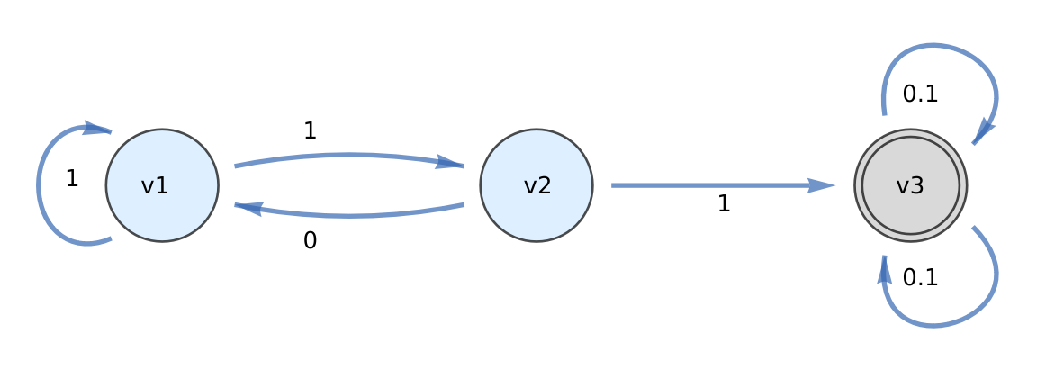
V = (v₁, v₂, v₃),
Σ = {0, 1},
s = v₁,
F = (v₁, v₂),
δ(v₁,0) = v₂ δ(v₁,1) = v₁,
δ(v₂,0) = v₃ δ(v₂,1) = v₁,
δ(v₃,0) = v₃ δ(v₃,1) = v₃.
Note that in the diagram, states v₁ and v₂ are the accepting states. If this DFA is presented with the input string 011010011, it will go through the following states: v₁, v₂ v₁, v₁, v₂, v₁ v₂, v₃, v₃, v₃.
Hence, the string is not admissible because it is not in the language accepted by this automaton. The language it accepts, as a careful look at the diagram reveals, is the set of all binary strings that contain no successive zeroes.
Now we employ Mathematica to define and plot the corresponding atomation. First, we define the states:
Customary define vertex shape function for double circles
In this section, we concentrate our attention on probabilistic problems and show by examples how some problems can be solved in a straightforward way if we apply the finite state machine approach. As a side affect, since we obtain directly the probability generating functions of the random variables involved, we have direct access to the moments without actual knowledge of the distributions. The demonstrated technique is especially beneficial for solving probabilistic waiting time problems when the object of interest is a specific sequence of runs, called the patterns.
In the second part of this section, we consider problems with two stopping patterns, which could be extended for multiple choices. Such kind of problems are usually solved using advanced techniques---the methods of Markov chains (see next section), martingales, or multiple gambling teams (see Feller's book and Pozdnyakov's article). Instead, we show that techniques based on the finite state machine approach are adequate for solving such kind of problems.
To solve this problem, we need a mathematical model---a sample space that consists of all possible outcomes. We list the outcomes in rows according to the number of tosses needed to get three sequential consecutive head, after that the process is terminated. For instance, HTHHH is such outcome for five flips, where H stands for head and T---for tail. Since there is no (fixed) number that assures that the number of trials does exceed it, the sample space is infinite---it contains all finite strings over the alphabet { T, H } ending with three head. There are infinitely many outcomes, but there are no outcomes that represent infinitely many trials.
A finite state automaton (FSA) or machine is an excellent tool to handle such kind of problems. We consider the transition diagram for the FSA accepting all strings with three consecutive head. Let us denote by p the probability to get head, and q = 1- p to get tail.
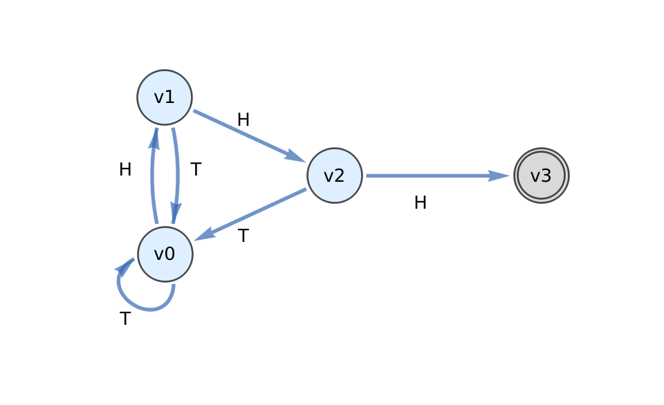
Note that the state v₃ is the accepting state and the game is over since we obtain the required number of head. Let di (i = 1, 2, 3) be the expected duration of the game from any state i, and d = d₀ be the expected value of X, which corresponds to the duration of the game from the start vertex v₀. We denote by pik the probability of getting from state i to state k in one step. Then for every i = 0, 1, 2, 3, we get the equation:
G[z_] = p^3 z^3 /(1 - (1-p)*z - p*(1-p)*z^2 -(1-p)*p^2 * z^3);
D[G[z], z]
G[z_] := (p^3 z^3)/(1 - q z - q p z^2 - q p^2 z^3);
FullSimplify[D[G[z], z] /.z->1]
Wolfram code summarizes the above calculations. Start by clearing existing definitions
Let us choose letters at random from an alphabet of n letters, one at a time. We continue sampling until the last m letters form a given pattern or stopping string. The number of trials to see the pattern is called the waiting time. For instance, we flip a coin until we see the pattern P = HHH; or we roll a die repeatedly until we get (1,2,3). More generally, how many times do you need to invoke a random number generator to observe a particular sequence of numbers?
Let P be a pattern---a given sequence of letters. We say that there is an overlap of length r if the last r letters of P match its first r letters. We set εr = 1 in this case and 0 otherwise. For example, the pattern HHH has 3 overlaps (so ε₁ = ε₂ = ε₃ = 1), but the stopping sequence (1,2,3) has no overlaps except itself (ε₁ = ε₂ = 0, ε₃ = 1). Let m be the length of the pattern, and n be the number of letters in the alphabet. In what follows, we assume that every letter is equally likely to be chosen. Next, we introduce the conditional probabilities
With the generating function at hand, we differentiate it and set z = 1 to obtain the mean, μ, and variance, σ², of the waiting time:
\[Epsilon][r_, pattern_] := If[StringTake[pattern, r] == StringTake[pattern, -r], 1, 0]
variance = (D[phiZ, {z, 2}] /. z -> 1) + mean - mean^2
142
We summaries expected waiting time for flipping a fair coin:
"HHH" → 14,
"HHT" → 10,
"HTH"" → 20,
"HTT"" → 8,
"THH"" → 18,
"THT"" → 12,
"TTH"" → 6,
"TTT"" → 14.
These values are indeed the expected waiting times for each pattern to occur, calculated by using the transitions between states in the corresponding finite state machine. You can use these values to understand how likely or unlikely certain sequences are to appear in a series of coin flips.
■
Multi pattern stopping problems
So far we considered problems with one final state. In what follows, we discuss a wide class of problems about waiting times with multiple stopping patterns. Waiting time distributions generated by compound patterns are rather large and include, for example, geometric and negative binomial distributions. Waiting times distributions have been used in various areas of statistics and some applications in reliability, sampling inspections, quality control, DNA sequencing, and others.Consider an experiment with only countable many outcomes when every trial is performed repeatedly. For instance, flipping a coin n times (n can be any positive integer), we obtain a binary sequence of two letters---H and T. We are looking for the expected number of tosses and probability till one of two given sequences of patterns observed first. Since our goal is not to present the general results of waiting time distribution (You can trace this subject in the article Pozdnyakov et al), but rather give an exposition of available tools, we encourage the reader to go with us over examples and then solve exercises.
Now we analyze the case when there are two or more stopping sequences, denoted by P₁, P₂, … , Pk. We present a technique for efficient determination which of multiple candidate sequences (e.g. HHH, HHT, THH) is more likely to appear first in a stream of fair or biased coin flips. This clever algorithm was discovered by the British--American mathematician John Conway (1937--2020), which was indirectly presented in the chapter on Pattern Matching and Penney's Game of the Berlekamp, E.R., Conway, J.H., Guy, R.K. book.
For any pair of patterns, Pi and Pj, Jphn Conway introduced the so called leading numbers that are defined as follows:
For given k patterns of the same length m from an alphabet with n letters, the mean waiting time and the stopping probabilities are \begin{equation} \label{E87.4} \mu = \left( \sum_{i=1}^k x_i \right)^{-1} , \qquad \pi_j = x_j \left( \sum_{i=1}^k x_i \right)^{-1} , \quad j=1, \ldots , k, \end{equation} where x₁, x₂, … , xk satisfy the linear system of equations \begin{equation} \label{E87.5} \sum_{i=1}^k e_{i,j} x_i = n^{-m} , \qquad \mbox{with} \quad e_{i,j} \stackrel{\tiny def}{=} \sum_{r=1}^m \epsilon_r (i,j) n^{r-m} , %\quad i,j=1,2,\ldots , k. \end{equation} i, j = 1, 2, … , k.
Each pattern has a "leading number" (also called a "successor function" or sometimes a "matching matrix") that determines how patterns interfere with each other, Eq.(5). For each pair of patterns, say A and B, the Conway algorithm includes five steps.
- For each pattern, construct a "predecessor tree" by checking suffix-prefix matches. You create a value for how often one pattern interferes with another.
- Assign a leading numbers to each pair of patterns: \[ \varepsilon_r (A,B)= \begin{cases} 1, & \mbox{if there is an overlap of length} \ r, \\ 0, & \mbox{if there is no overlap of length} \ r. \end{cases} \tag{5} \]
- Calculate the Conway number for each pair of patterns: \[ \mbox{Conway number}(A, B) = \sum_{r=1}^m \varepsilon_r (A, B) \cdot 2^{r} , \] where εi = 1 if the length i suffix of B matches the prefix of A.
- Calculate the expected number of flips ubtil first appearance: \[ \begin{split} \mu (A, B) &= \left[ C(A, A)\, C(B, B) - C(B, A)\, C(A,B) \right] \\ &\times \left[ \frac{1}{C(B, B) - C(A, B)} + \frac{1}{C(B, A) - C(A,A)} \right] . \end{split} \] where C(A, B) is the Conway number for patterns A and B.
- Evaluate the probability to win for each pattern: \[ \Pr [A] = \frac{C(B, B) - C(A, B)}{C(B, B)\,C(A, A) - C(B, A)\, C(A, B)} \cdot \mu , \] \[ \Pr [B] = 1 - \Pr [A] . \]
We flip a fair coin repeatedly and consider the number of times it takes for particular triplets (TTH, or HHH etc.) to appear. If we flip it just three times then each of the eight triplets is equally likely to show up. But if we persist, and ask questions about time to first appearance of each pattern, or about the likelihood of seeing one pattern before another, then inequalities emerge. Not always, by symmetry we expect either of three head or three tail to be produced before the other, but it turns out that any of other triplets is likely to appear before these two. Every (i, j)th entry in the following 8×8-matrix contains the probability that triplet i occurs in a sequence of coin flips before triplet j. The exercise 3 asks you to verify these probabilities.
| HHH | HHT | HTT | HTH | THT | THH | TTH | TTT | |
|---|---|---|---|---|---|---|---|---|
| HHH | --- | ½ | ⅖ | ⅖ | 5/12 | ⅛ | 3/10 | ½ |
| HHT | ½ | --- | ⅔ | ⅔ | ⅝ | ¼ | ½ | 7/10 |
| HTT | ⅗ | ⅓ | --- | ½ | ½ | ½ | ¾ | ⅞ |
| HTH | ⅗ | ⅓ | ½ | --- | ½ | ½ | ⅜ | 7/12 |
| THT | 7/12 | ⅜ | ½ | ½ | --- | ½ | ⅓ | ⅗ |
| THH | ⅞ | ¾ | ½ | ½ | ½ | --- | ⅓ | ⅗ |
| TTH | 7/10 | ½ | ¼ | ⅝ | ⅔ | ⅔ | --- | ½ |
| TTT | ½ | 3/10 | ⅛ | ½ | ⅖ | ⅖ | ½ | --- |
SequenceProbability["HTH", "HHH"]
SequenceProbability["HTH", "THH"]
Similarly to average waiting time, we get
=====================================================
| HHH | HHT | HTT | HTH | THT | THH | TTH | TTT | |
|---|---|---|---|---|---|---|---|---|
| HHH | \( \frac{1}{p} + \frac{1}{p^2} + \frac{1}{p^3} \) | 7 | 14/5 | 17/5 | 35/6 | 7/2 | 28/9 | 7/2 |
| HHT | 7 | --- | ⅔ | ⅔ | ⅝ | ¼ | ½ | 7/10 |
| HTT | ⅗ | ⅓ | --- | ½ | ½ | ½ | ¾ | ⅞ |
| HTH | ⅗ | ⅓ | ½ | --- | ½ | ½ | ⅜ | 7/12 |
| THT | 35/6 | ⅜ | ½ | ½ | --- | ½ | ⅓ | ⅗ |
| THH | ⅞ | ¾ | ½ | ½ | ½ | --- | ⅓ | ⅗ |
| TTH | 7/10 | ½ | ¼ | ⅝ | ⅔ | ⅔ | --- | ½ |
| TTT | ½ | 3/10 | ⅛ | ½ | ⅖ | ⅖ | ½ | --- |
Let us consider one entry, say "5/12" of pattern HHH vs THT. To determine the probability of seeing HHH before THT, we plot a graph of transition probabilities for corresponding DFA.
pH = 1/2; equations = { pT == 1/2 + 1/2 pT + 1/2 pH + 1/2 pHH, pHH == 1/4 + 1/2 pTH, pTH == 1/2 pT, pHHH == 1/2 pHH, pTHT == 1/2 pTH }; solutions = Solve[equations, {pT, pHH, pTH, pHHH, pTHT}]
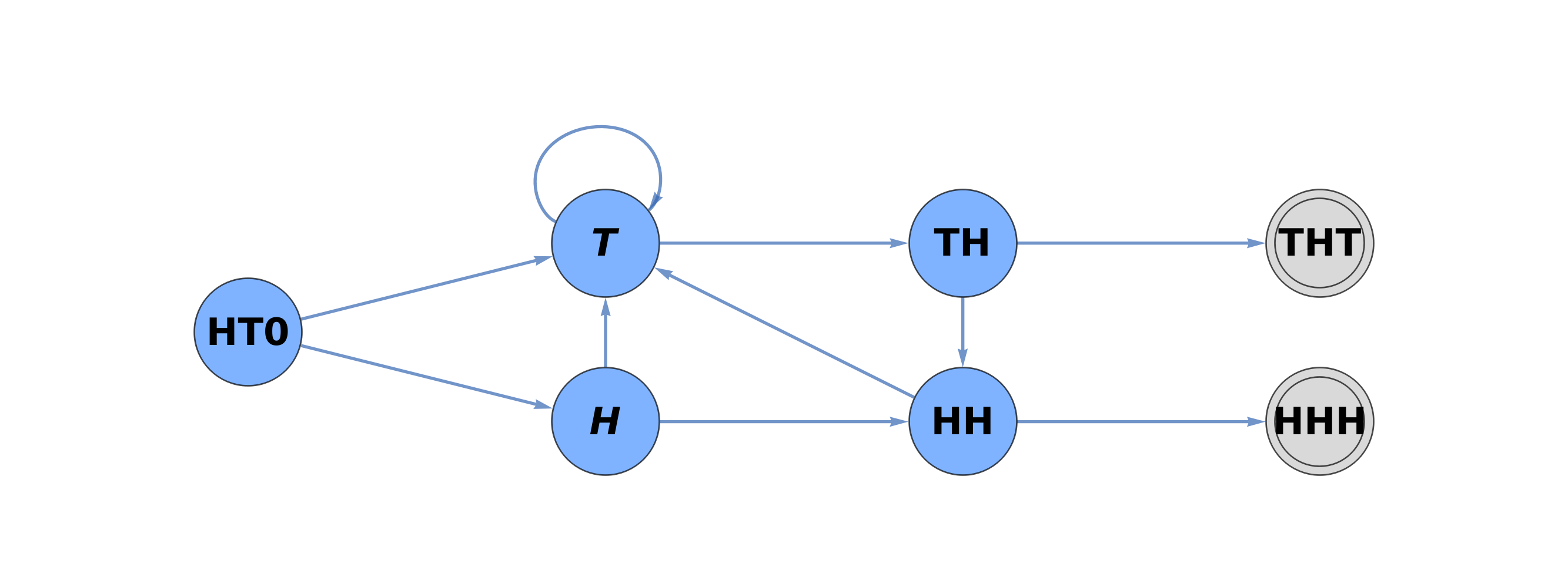
It should be noted that all states except final states (HHH and THT) should have two outgoing arrows corresponding two outcomes due to flipping a coin---either HEAD or Tail.
For two stopping states, HHH (set i = 1) and THT (set i = 2), we introduce leading numbers: \[ \varepsilon_r (1,1) = 1 \quad (r = 1, 2, 3), \qquad \varepsilon_1 (2,2) = 1, \quad \varepsilon_3 (2,2) = 1. \] All other leading numbers are zeroes (RJB explains). The corresponding coefficients are \[ e_{1,1} = 1 + \frac{1}{2} + \frac{1}{4} = \frac{7}{4}, \qquad e_{2,2} = 1 + \frac{1}{4} = \frac{5}{4} . \] This leads to system of two equations: \[ \frac{7}{4}\, x_1 = \frac{1}{8} , \qquad \frac{5}{4}\, x_2 = \frac{1}{8} . \] You don't need a computer to solve these two equations: \[ x_1 = \frac{1}{14} , \quad x_2 = \frac{1}{10} \qquad\Longrightarrow \qquad x_1 + x_2 = \frac{6}{35} . \]
Luckily, the captured man had a laptop with a software algebra system, and the prisoner was able to make use of it. The computer scientist spent a few minutes on the problem and asked the pirate to use letters on all faces (which would make the die more attractive). He suggested and the captain agreed to use letters L, I, V, E, D, and A on it, and let the deciding words to be LIVE or DEAD. What is the expected number of rolls for each of three words?
Solution. First, we draw a DFA that simulates appearance of the five letters. Note that solid lines indicate movements with probability ⅙ and dotted lines show transitions with different probabilities (mostly ½ by default, but some with ⅔). There are two accepting states.

Then we calculate the expected number of rolls to reach one of the final states. Denoting this number by d, we derive the following equation \[ d=1+ \frac{2}{3}\,d + \frac{1}{6}\, d_l +\frac{1}{6}\,d_k , \] where d₁ and dk are expected numbers to reach the final states from states ``L'' and ``K,'' respectively. These expected values are also expressed via expected values to get to the final states from other states: \[ d_l = 1 +\frac{1}{6} \,d_l + \frac{1}{6} \,d_k + \frac{1}{6} \,d_{li} + \frac{1}{2} \,d , \qquad d_k = 1 +\frac{1}{6} \,d_l + \frac{1}{6} \,d_{k} + \frac{1}{6} \,d_{ki} + \frac{1}{2} \,d . \] Similarly, we obtain \begin{align*} d_{li} &= 1 +\frac{1}{6} \,d_l + \frac{1}{6} \,d_k + \frac{1}{6} \,d_{liv} + \frac{1}{2} \,d , \quad &d_{ki} &= 1 +\frac{1}{6} \,d_{kil} + \frac{1}{6} \,d_k + \frac{2}{3} \,d , \\ d_{liv} &= 1 +\frac{1}{6} \,d_l + \frac{1}{6} \,d_k + \frac{1}{2} \,d , \quad &d_{kil} &= 1 +\frac{1}{6} \,d_{li} + \frac{1}{6} \,d_k + \frac{1}{2} \,d . \\ \end{align*} Solving this system of equations, we obtain the expected number of rolls to finish the game: \[ d=\frac{279936}{431} \approx 649.50348 \quad\mbox{or about 650 rolls.} \] Now we consider the case when there is only one stopping pattern---either KILL or LIVE. Since they are similar, we draw only one DFA:
Solving the following system of equations \begin{align*} d&= 1+\frac{5}{6}\, d +\frac{1}{6}\, d_{l} , \quad &d_{l} &= 1 +\frac{1}{6}\, d_{l} +\frac{1}{6}\, d_{li} + \frac{2}{3}\, d , \\ d_{li} &= 1+ \frac{1}{6}\, d_{liv} + \frac{1}{6}\, d_{l} + \frac{2}{3}\, d , \quad &d_{liv} &= 1 + \frac{1}{6}\, d_{l} + \frac{2}{3}\, d , \end{align*} for d, the expected value to reach the final state LIVE, we obtain \[ d=1296 . \] The probability for the machine to be at a particular state (there are nine of them) depends on the number of rolls. However, their numerical values are not our immediate concern. Instead, we are looking for the case when the number of trials increases without bounds trying to evaluate the `"ultimate'' probability for infinite sequence of letters (if they are not terminated by two absorbing states). We denote by pk, pl, pki, pli, pkil, and pliv the limiting ``probabilities'' to reach states ``K,'' ``L,'' ``KI,'' ``LI,'' ``KIL,'' ``LIV,'' respectively.
We can arrive to state ``K'' either from the starting state (with probability ⅙), or from the same state ``K'' (with probability ⅙), or from the state ``L'' (with probability ⅙), or from the state ``LI'' (with probability ⅙), or from the state ``LIV'' (with probability ⅙), or from the state ``KI'' (with probability ⅙), or from the state ``LIV'' (with probability ⅙). So we have the equation \[ p_k = \frac{1}{6} + \frac{1}{6} \, p_k + \frac{1}{6} \, p_l + \frac{1}{6} \, p_{ki} + \frac{1}{6} \, p_{kil} + \frac{1}{6} \, p_{li} + \frac{1}{6} \, p_{liv} . \] Similarly, we can reach the state ``L'' from the starting state and states ``K,'' ``LI,'' and ``LIV,'' all with the same probability ⅙. This observation we translate into the equation \[ p_l = \frac{1}{6} + \frac{1}{6} \, p_k + \frac{1}{6} \, p_l + \frac{1}{6} \, p_{li} + \frac{1}{6} \, p_{liv} . \] For other states we get similarly \[ p_{li} = \frac{1}{6} \, p_l + \frac{1}{6} \,p_{kil} , \quad p_{liv} = \frac{1}{6} \, p_{li} , \quad p_{ki} = \frac{1}{6} \, p_{k} , \quad p_{kil} = \frac{1}{6} \, p_{ki} . \] Hence, we need to find pkil and pliv from this system of algebraic equations because the probabilities to reach the final states are just ⅙ times these probabilities. When a CAS is available, it is not hard to find these probabilities to obtain \[ p_{kil} = \frac{216}{28339} , \quad p_{liv} =\frac{215}{28339} , \] Since the odds of the states KILL vs LIVE are 216 : 215, we get the following probabilities: \[ \Pr [\mbox{KILL}] =\frac{216}{215+216} = \frac{216}{431} \approx 0.5011600928, \quad \Pr [\mbox{LIVE}] =\frac{215}{431} \approx 0.4988399072 . \] Note that there KILL (or LIVE) is the event that a run of consecutive letters KILL (or LIVE occurs before a run of consecutive letters LIVE (or KILL).
The case LIVE vs DEAD can be treated in a similar way. However, we present its solution in the following example, using another technique.
The prisoner was able to convince the pirate to use his die idea by telling him that it would be much more elegant to have 6 full letters on the die, rather than 5 and a blank. The pirate agreed, and he started rolling. The result of 474 rolls was:
vleideedeilelvdllidlvevvdieeaididvldevelvadeeevieaivavidei
eiiiaaddaddivalaeaeeivvilvvlveavaldaeedeilivaveaveleealddl
veaeividevevlldadelddlivavvialvaleeeedaleailvlvvlvilalilai
aleallaevaidveaidddlladdlalilvideiladldeviivlvddadvlvvvlei
vevivllaveldvlvavvevilaiavidvvvlelleldevdldaleiivldveliiee
iialevaledvvlivvvdivdead
Even with a slight advantage, the computer scientist will still lose in the long run. Being an enterprising man, the pirate offered him one last chance to save his life. He noticed that the prisoner was an excellent computer scientist and he had some ideas for a start-up company. If the prisoner would work for 12 hours a day, 7 days a week, he would be spared and if the company was successful, he would be rewarded with 5% of all profits. The computer scientist was shocked! This was a better offer than where he was working before! ■
Now we calculate the expected number of rolls, denoted by $d$, to see the run of DEAD by solving the following system of algebraic equations: \begin{align*} d&=1+\frac{5}{6}\,d +\frac{1}{6}\,d_{D} , \quad &d_{D} &= 1+\frac{1}{6}\,d_{D} +\frac{2}{3}\,d + \frac{1}{6}\,d_{DE} , \\ d_{DE} &=1+\frac{1}{6}\,d_{D} +\frac{2}{3}\,d + \frac{1}{6}\,d_{DEA} , \quad &d_{DEA} &=1+\frac{5}{6}\,d . \end{align*}
- Find the expected number of flips of a biased coin to see r (r ≥ 3) consecutive head by deriving a corresponding enumerator.
-
Let M = { V, Σ, δ, v₀, F } be a DFA, where V = { v₀, v₁, v₂, v₃ }, Σ = {0, 1}, F = { v₃ },
and the transition function is given by the following table:
State 0 1 v₀ v₀ v₁ v₁ v₁ v₂ v₂ v₁ v₃ v₃ v₃ v₁ Which of the following strings are in L(M)? (a) ε
(b) 001101,
(c) 1110,
(d) 11011. -
Find the mean waiting time and verify stopping probabilities for each pair of
the eight triplets when flipping a fair coin in the table.
HHH HHT HTT HTH THT THH TTH TTT HHH --- ½ ⅖ ⅖ 5/12 ⅛ 3/10 ½ HHT ½ --- ⅔ ⅔ ⅝ ¼ ½ 7/10 HTT ⅗ ⅓ --- ½ ½ ½ ¾ ⅞ HTH ⅗ ⅓ ½ --- ½ ½ ⅜ 7/12 THT 7/12 ⅜ ½ ½ --- ½ ⅓ ⅗ THH ⅞ ¾ ½ ½ ½ --- ⅓ ⅗ TTH 7/10 ½ ¼ ⅝ ⅔ ⅔ --- ½ TTT ½ 3/10 ⅛ ½ ⅖ ⅖ ½ --- - A coin is tossed successively until either two consecutive head occur in a row or four tail occur in a row. What is the probability that the sequence ends with two consecutive head? What is expected number of tosses for this event?
- A coin is tossed successively until one of the following patterns is observed: either a run of H's of length m or a run of T's of length n. We know from Example~\ref{M582.3} that the expected waiting time of the run of H's is 2m+1 - 2, while for the run of T's it is 2n+1 - 2. Find the expected number of tosses until either of these two runs happens for the first time and show that for a fair coin this number is \[ \left( \frac{1}{2^{m+1} -2} +\frac{1}{2^{n+1} -2} \right)^{-1} = \frac{2^{n+m} - 2^{n} - 2^{m} +1}{2^{n-1} + 2^{m-1} -1} \,. \]
-
Suppose you flip a fair coin without stopping, what is the average
waiting time until the first occurrence of the pattern occurs? Write
the enumerator for each event.
-
HHHHH,
-
HTHTH,
-
HHHTH,
- HHHHT .
-
HHHHH,
- What is the probability that in a stochastic sequence of head (H) and tail (T) the pattern HHHHT appears earlier than HHHTH? Assume that tail lands with probability q.
-
(a)
On average, how many times do you need to choose digits from the alphabet
Σ = { 0, 1, … , 9 } (taken randomly with replacement) to see
4-long sequence (i, i, i, i), i ∈ Σ?
(b) A pseudo-random generator produces r-tuples of integers (i₁, i₂, … , ir ) from the alphabet Σ = { 0, 1, … , 9 }. What is expected waiting time (measured in the number of calls of the random generator) for the sequence (i, i, … , i)? DFA: - The goal of this exercise is to show that some waiting time problems may have counterintuitive solutions. Given two sequences of patterns, HTHT and THTT, a coin is flipped repeatedly until one of the patterns appears as a run; what pattern win? Find the expected number of tosses needed to see a winner; also, determine the expected running time (=number of flips) for each of the patterns. As a check on your answers for a fair coin: the odds are 9 to 5 in favor of getting HTHT first, though its expected number of tosses till first arrival is 20, whereas the pattern THTT needs only 18 flips on the average.
- Suppose, for instance, that A flips a coin until she observes either HHHTH or HTHTH, while B flips another coin until he observes either HHHHT or HHHTH. Here H stands for head and T---for tail. It is assumed that both coins have the same probability p of head on each trial. For what p the average waiting times for A and for B will be the same?
- Berlekamp, E.R., Conway, J.H., Guy, R.K., Winning Ways for Your Mathematical Plays, Second edition, A K Peters/CRC Press, 2001.
- Blom, Gunnar and Thorburn, Daniel, How many random digits are required until given sequences are obtained?, Journal of Applied Probability, 19, 518 -- 531, 1982.
- Blom, Gunnar, On the mean number of random digits until a given sequence occurs, Journal of Applied Probability, 1982, Vol. 19, pp. 136--143.
- Collings, S., Coin sequence probabilities and paradoxes, Bulletin of the Institute of Mathematics and its Applications, Vol. 16, November--December, 1982, pp. 227--232.
- Conway, J., Game pf :ife Explanation.
- Feller, William, An Introduction to Probability Theory and its Applications, 3rd Ed., John Wiley & Sons, New York, 1968.
- Gardner, M., The Colossal Book of Short Puzzles and Problems, W. W. Norton & Company, 2005.
- Hopcroft, John E., Motwasni, Rajeev, and Ullman, Jeffrey D., Introduction to Automata Theory, Languages and Computation, 3rd Ed., Addison Wesley, Boston, MA, 2007.
-
Knuth, D.E., The Art of Computer Programming, Vol. 1, Fundamental Algorithms, 3rd Edition, Addison-Wesley Professional, 1997.
Vol.2, Seminumerical Algorithms.
Vol.3, Sorting and Seaching. -
Mitzenmacher, M. & Upfal, E., Probability and Computing
Randomized Algorithms and Probabilistic Analysis, Cambridge University Press, 2005.
See also Probability and Computing. - Nishiyama, Y., Pattern matching probabilities and paradoxes---A a new variation on Penney's coin game, Osaka Keidai Ronshu, Vol. 68, No. 4, November, 2012.
- Nishiyama, Y., Pattern matching probabilities and paradoxes as a new variation on Penney's coin game, International Journal of Pure and Applied Mathematics (JPAM), Volume 59, No 3, 2010.
- Pozdnyakov, Vladimir and Kulldorf, Martin, Waiting times for patterns and a method of gambling teams, The American Mathematical Monthly, 113, No. 2, 134 -- 143, 2006.
- Sudkamp, Thomas A., Languages and Machines, An Introduction to the Theory of Computer Science, 3rd Ed., Addison-Wesley, Reading, MA, 2006.