Introduction to Linear Algebra
1. Systems of Linear Equations
- Introduction
- Linear systems
- Vectors
- Linear combinations
- Matrices
- Planes in ℝ³
- Reduced Row-Echelon Form
- Equation A x = b
- Sensitivity of solutions
- Linear independence
- Plane transformations
- Space transformations
- Linear transformations
- Affine maps
- Exercises
- Answers
2. Matrix Algebra
- Introduction
- Manipulation of matrices
- Partitioned matrices
- Block matrices
- Matrix operators
- Determinants
- Cofactors
- Cramer's rule
- Equivalent matrices
- Elimination: A = L U
- PLU factorization
- Reflection
- Givens rotation
- Special matrices
- Exercises
- Answers
3. Vector Spaces
- Introduction
- Motivation
- Vector spaces
- Bases
- Dimension
- Coordinate systems
- Linear transformations
- Change of basis
- Matrix transformations
- Compositions
- Isomorphisms
- Dual transformations
- Quotient spaces
- Rank
- Solving A x = b
- Exercises
- Answers
4. Eigenvalues, Eigenvectors
- Introduction
- Characteristic polynomials
- Companion matrix
- Algebraic and geometric multiplicities
- Minimal polynomials
- Eigenspaces
- Where are eigenvalues?
- Eigenvalues of A B and B A
- Generalized eigenvectors
- Similarity
- Diagonalizability
- Self-adjoint operators
- Exercises
- Answers
5. Euclidean Spaces
- Introduction
- Four spaces
- Euclidean space
- Bilinear transformations
- Norm and distance
- Matrix norms
- Dual norms
- Dual transformations
- Examples of transformations
- Orthogonality
- Gram--Schmidt Process
- Orthogonal matrices
- Self-adjoint matrices
- Unitary matrices
- Projection operators
- QR-decomposition
- Least Square Approximation
- Quadratic forms
- Exercises
- Answers
6. Canonical forms
- Introduction
- 2D decomposition
- 3D decomposition
- Projectors
- Direct-sum decompositions
- Cyclic decompositions
- Symmetric matrices
- Pseudoinverse
- URV-decomposition
- LU-decomposition
- QR-decomposition
- Cholesky decomposition
- Schur decomposition
- Positive matrices
- Roots
- Polar factorization
- Spectral decomposition
- CUR decomposition
- Exercises
- Answers
7. Applications
- Introduction
- Circles along curves
- TNB frames
- GPS problem
- Coriolis acceleration
- Poisson equation
- Graph theory
- Error correcting codes
- Electric circuits
- FSA
- Markov chains
- Cryptography
- Wave-length transfer matrix
- Computer graphics
- Linear Programming
- Hill's determinant
- Fibonacci matrices
- Discrete dynamic systems
- Discrete Fourier transform
- Fast Fourier transform
- Curve fitting
- Answers
Miscellany
- Introduction
- Circles along curves
- TNB frames
- Differential forms
- Calculus
- Vector representations
- Matrix representations
- Change of basis
- Orthonormal Diagonalization
- Generalized inverse
- Differential forms
Preliminaries
- Complex Number Operations
- Sets
- Polynomials
- Polynomials and Matrices
- Computer solves Systems of Linear Equations
- Location of Eigenvalues
- Power Method
- Iterative Method
- Similarity and Diagonalization
Glossary
Reference

This Book is licensed under Creative Commons Attribution-NonCommercial-NoDerivs 3.0 Unported License
The material of this section is based on solvability section. Therefore, the reader is advised to study this section first before reading underlying material.
Least Square Approximation
When a linear system A x = b satisfies Corollary 5 of dot section, a perfect solution exists because b lies entirely within the column space 𝒞(A). However, in real-world applications—such as experimental data fitting and overdetermined systems (m > n)—measurement noise or unmodeled dynamics often pull the target vector b outside of 𝒞(A).
Because no true solution exists, our objective shifts from finding a perfect solution to finding an optimal approximation that minimizes the Euclidean norm of the residual vector r = b − A x.
The distance between b and any vector in the column space is minimized when the residual vector r = b − A x̂ is strictly orthogonal to the column space itself (r ⊥ 𝒞(A)).
figure x̂By Theorem 15 of dot section, the orthogonal complement of the column space is the left null space (𝒞(A)⊥ = ker(A✶)). Therefore, the optimality condition dictates that the residual must live in the left null space:
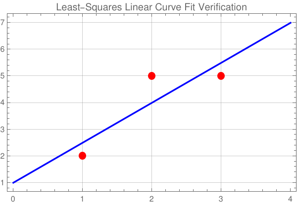
Consider three experimental data points (x, y): (1, 2), (2, 5), and (3, 5). We want to fit a straight line y = m x + c to these points. This overdetermined system yields three equations for two unknowns:
Step 1: Compute the Normal Equation Matrix Aᵀ A and Vector Aᵀ b:
Step 2: Solve the System AᵀA x̂ = Aᵀ b:
Inverting the 2 × 2 matrix yields:
Multiplying to find the optimal parameter weights x̂:
Conclusion: The unique least-squares optimal line is y = 1.5x + 1.0. The projected optimal coordinates on the column space are A x̂ = [2.5, 4.0, 5.5]^{\mathrm{T}}$, yielding a minimized residual error vector r = [-0.5, 1.0, -0.5]ᵀ.
■Option A: Direct Algebraic Solver via Normal Equations: