
Introduction to Linear Algebra
Complex Variables
- Introduction
- Real numbers
- Complex numbers
- Polar representation
- Riemann's sphere
- Topology
- Integration
- Differentiation sphere
- Conformal maps
- Reduced Row-Echelon Form
- Equation A x = b
- Sensitivity of solutions
- Linear independence
- Plane transformations
- Space transformations
- Linear transformations
- Affine maps
- Exercises
- Answers
Series and Limits
- Introduction
- Definition of derivative
- Geometric meaning
- Properties Matrix operators
- Determinants
- Cofactors
- Cramer's rule
- Equivalent matrices
- Elimination: A = L U
- PLU factorization
- Reflection
- Givens rotation
- Special matrices
- Exercises
- Answers
Differentiation
- Introduction
- Definition of derivative
- Geometric meaning
- Properties Compositions
- Derivative of inverse
- Power rule
- Right and Left-hand derivatives
- Higher order derivatives
- Infinitesimals
- Differentials
- Extrema of a real-valued functions
- Fermat's and Rolle's theorems
- Lagrange theorem
- de l'Hospital's rule
- Dual transformations
- Direct sums
- Quotient spaces
- Rank
- Solving A x = b
- Exercises
- Answers
Integration
- Introduction
- Riemann integral
- Area and integral
- Properties of integration
- Primitive functions
- Fundamental theorem of calculus
- Integration by parts
- Indefinite integrals
- Improper integrals
- Improper integrals II
- Mean value theorems
- Double integral
- Polar coordinates
- Self-adjoint operators
Vector Calculus
- Introduction
- Vector fields
- Paths
- Line integrals
- Answers
- Inner product
- Norm and distance
- Matrix norms
- Dual norms
- Dual transformations
- Examples of transformations
Tensors
- Introduction
- LU-decomposition
- QR-decomposition
- Cholesky decomposition
- Schur decomposition
- Positive matrices
- Roots
- Polar factorization
- Spectral decomposition
- Singular values
- SVD <
- Pseudoinverse
- Exercises
- Answers
Calculus of Variations
- Introduction
- GPS problem
- Poisson equation
- Graph theory
- Error correcting codes
- Electric circuits
- Markov chains
- Cryptography
- Wave-length transfer matrix
- Computer graphics
- Linear Programming
- Hill's determinant
- Fibonacci matrices
- Discrete dynamic systems
- Discrete Fourier transform
- Fast Fourier transform
- Curve fitting
Classical mechanics
- Introduction
- Similar matrices
- Diagonalization
- Sylvester formula
- The Resolvent method
- Polynomial interpolation
- Positive matrices
- Roots <
- Pseudoinverse
- Exercises
- Answers
Quantum mechanics
- Introduction
- Circles along curves
- TNB frames
- Tensors
- Tensors in ℝ³
- Tensors & Mechanics
- Differential forms
- Calculus
- Vector Representations
- Matrix Representations
- Change of Basis
- Orthonormal Diagonalization
- Generalized Inverse
- Differential forms
Preliminaries
- Complex Number Operations
- Sets
- Polynomials
- Polynomials and Matrices
- Computer solves Systems of Linear Equations
- Location of Eigenvalues
- Power Method
- Iterative Method
- Similarity and Diagonalization
Glossary
Reference

This Book is licensed under Creative Commons Attribution-NonCommercial-NoDerivs 3.0 Unported License
Rational Numbers
A real number that is not rational is called irrational. Irrational numbers include the square root of 3 (∛3), π ≈ 3.1415925…, e ≈ 2.71828…, and the golden ratio (φ = (1 + ∛5)/2 ≈ 1.61803…). Since the set of rational numbers is countable, and the set of real numbers is uncountable, almost all real numbers are irrational. The field of rational numbers is the unique field that contains the integers, and is contained in any field containing the integers.
The system of rational numbers is ordered, i.e. if we have two different numbers 𝑎 and b of this system, one of them is greater than the other. Also, if 𝑎 > b and b > c, then 𝑎 > c, when 𝑎, b, and c are numbers of the system.
Further, if two different rational numbers 𝑎 and b are given, we can always find another rational number greater than the one and less any two different rational of rational numbers creater than the one and less then the other. It follows from this that between any two different rationak there are an infinite number of rational numbers.
Real numbers
The extension of the idea of number 3. Irrational Numbers. from the rational to the irrational is as natural,, if not as easy, as is that from the positive integers to the fractional and negative rational numbers.
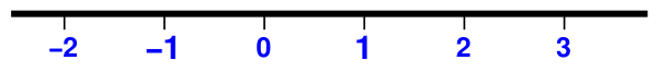
There are two familiar ways to represent real numbers. Geometrically, they may be pictured as the points (abstract objects of zero size) on a line, once the two reference points corresponding to 0 and 1 have been picked. For computation, however, we represent a real number as an infinite decimal, consisting of an integer part and the sign (plus or minus), followed by infinitely many decimal places:
On a straight line L, we take any segment of this line as unit of length, a definite point of the line as origin or zero point, and the directions of right and left for the positive and negative senses. To every rational number corresponds a definite point on the line. If the number is an integer, the point is obtained by taking the required number of unit segments one after the other in the proper direction. If it is a fraction ±p/q, it is obtained by dividing the unit of length into q equal parts and taking p of these to the right or left according as the sign is positive or negative. These numbers are called the measures of the corresponding segments, and the segments are said to be commensurable with the unit of length. The points corresponding to rational numbers may be called rational points.
There are, however, an infinite number of points on the line L that are not rational points. Although we may approach them as nearly as we please by choosing more and more rational points on the line, we can never quite reach them in this way. The simplest example is the case of the points copnciding with one end of the diagonal of a square, the sides of which are the unit of length, when the diagonal lies along the line L and its other end coincides with any rational point.
Thus, without considering any other case of incommensurability, we see that the line L is infinitely richer in points than the system of rational numbers.
Hence, it is clear that if we desire to follow arithmetically all the properties of the straight line, the rational numbers are insuffucuent, and it will be necessary to extend this system by the creation of other numbers.
Recall that a rational number is any number that can be expressed as a fraction of integers and the denominator is not zero. Examples include all integers (which can be written as a fraction with a denominator of 1), terminating decimals (like 0.3), and repeating decimals (like 0.3(21) = 0.3212121…). The set of all rational mi,bers is denoted by ℚ. But if the decimal does not terminate or recur, the number is not the ratio of two whole numbers and is said to be irrational.
Dedekind's cut
We are going to describe Dedekind's method (1872) of introducing the irrational number, in its most general form, into analysis. Dedekind cuts, named after German mathematician Richard Dedekind (1831--1916), but previously considered by Joseph Bertrand, are а method of constructing the real numbers from the rational numbers.
Let us suppose that by some method or other we have divided all the rational numbers into two nonempty classes, a lower class A and an upper class B, such that every number α of the lower class is less than every number β of the upper class.
When this division has been made, if number α belongs to the class A, every number less than α does so also; and if a number β belongs to the class B, every number greater than β does bo also.
Three different cases can arise.
-
The lower class can have a greatest number and the upper class no smallest number.
This would occur, if, for example, we put the number 7 and every number less than 7 in the lower class, and if we put in the upper class all the numbers greater than 7.
-
The upper class can have a smallest number and the lower class no greatest number.
This would occur, if, for instance, we put the number 7 and all the numbers greater than 7 in the upper class, while in the lower class we put all the numbers less than 7.
It is impossible that the lower class can have a greatest number m, and the upper class a smallest number n, in the same division of the rational numbers; for between the rational numbers m and n there are rational numbers, so that our hypothesis that the two classes contain all the rational numbers is contradicted.
- The lower class can have no greatest number and the upper class no smallest rational number.
For example, let us arrange the positive integers and their squares in two rows, so that the squares are underneath the number to which they correspond. Since the square of a fraction in its lowest terms is a fraction whose numerator and denominator are perfect squares, we see that there are not rational numbers whose squares are 2, 3, 4, 5, 6, 7, …,
Since the polynomial n! f(x) has integer coefficients and all its monomials in x are of degree at least n (this positive integer will be specified later), every single derivative f(2k)(0) with 0 ≤ k ≤ n is an integer. Indeed, differentiating an expression of the form \( \displaystyle \quad \frac{a_j}{n!}\, x^{n+ j} , \quad \) with 𝑎j and j ≥ 0 integers, 2k-times with respect to x, the evaluation at x = 0 is nonzero only if 2k = n + j. For 2k = n + j we obtain the integer \( \displaystyle \quad \frac{a_j (2k)!}{n!} . \ \) Since f(x) = f(1 − x), we also have that every single derivative f(2k)(1) with 0 ≤ k ≤ n is an integer. A straightforward calculation yields
Elementary algebra is concerned with the application of the arithmetic operations (+, − *, and ÷) to symbols representing real numbers. However, there are difficulties with decimal representation that we need to think about. The first is that two different infinite decimals can represent the same real number, for according to well-known rules, a decimal having only 9's after some place represents the same real nuber as a different decimal ending with all 0's (such decimals are called finite or terminating):
Another difficulty with infinite decimals is that it is not immediately obvious how to calculate with them. For finite decimals or ratios of integers (that could be represented by infinite decimals with periodic fractional parts) there is no problem; in this case we just follow the usual rules---add/subtract or multiply/divide starting at the right-hand end:
To get around this, instead of calculating with the infinite decimal, we use its truncations to finite decimals, viewing these as approximations to the infinite decimals. For instance, the increasing sequence of finite decimals
The decimal representation of this sequence is not as simple as it was for the sequence representing e or π where each new decimal digit is added on. The sequence representing e + π may contain changes in two decimal laces. For instance, in the fifth step of the last row, the first decimal place changes from 7 to 8. Nevertheless, as we compute more and more places, the earlier part of the decimals in this sequence ultimately does not change any more, and in this way we get the decimal expansion of a new number; we then define the sum e + π to be this number. ■
As this example shows, even the simplest arithmetic operations with real numbers require an understanding of sequences and their limits. So you get an answer not at once, but rather by making closer and closer approximations to it.
ℝ as a field
We discuss properties of arithmetic operations (addition, subtraction, multiplication, and division) from formal algebraic prospective.
- Closure: For any two elements 𝑎, b in semigroup S, the result of the operation, 𝑎 • b, is also an element in S.
- Associativity: For all 𝑎, b, and c in group S, the equation (𝑎 • b) • c = 𝑎 • (b • c) holds.
- Identity element: There exists an element e in S, such that for all elements 𝑎 in S, the equation e • 𝑎 = 𝑎 • e = 𝑎 holds. This identity element is usually denoted by 1.
- Commutativity: For all 𝑎, b in S, 𝑎 • b = b • 𝑎.
- Closure: For any two elements 𝑎, b in A, the result of the operation, 𝑎 + b, is also an element in A.
- Associativity: For all 𝑎, b, and c in group A, the equation (𝑎 + b) + c = 𝑎 + (b + c) holds.
- Identity element: There exists an element e in A, such that for all elements 𝑎 in A, the equation e + 𝑎 = 𝑎 + e = 𝑎 holds. This element is usually denoted by zero.
- Inverse element: For each 𝑎 in A there exists an element b in A such that 𝑎 + b = b + 𝑎 = e (= 0), where e is the identity element (zero).
- Commutativity: For all 𝑎, b in A, 𝑎 + b = b + 𝑎.
The set ℝ, equipped with the usual addition "+" and multiplication "·" (also denoted by "•"), is a field. This means it satisfies the field axioms: commutative groups under addition, commutative monoid under multiplication with multiplicative inverses for nonzero elements, and distributively of multiplication over addition.
| name | addition | multiplication | ||
|---|---|---|---|---|
| associativity: | (𝑎 + b) + c = 𝑎 + (b + c) | (𝑎 • b) • c = 𝑎 • (b • c) | ||
| commutativity: | 𝑎 + b = b + 𝑎 | 𝑎 • b = b • 𝑎 | ||
| distributivity: | 𝑎 • (b + c) = 𝑎•b + 𝑎•c | (𝑎 + b) • c = 𝑎•c + b•c | ||
| identity: | 𝑎 + 0 = 𝑎 = 0 + 𝑎 | 𝑎•1 = 1•𝑎 = 𝑎 | ||
| inverses: | 𝑎 + (−𝑎) = 0 = (−a) + 𝑎 | 𝑎•𝑎−1 = 1 = 𝑎−1•𝑎 if 𝑎 ≠ 0 |
- Apostol, T.M., Calculus, Vol. 2: Multi-Variable Calculus and Linear Algebra with Applications to Differential Equations and Probability, Wiley; 2nd edition, 1991; ISBN-13: 978-0471000075.