Return to computing page for the first course APMA0330
Return to computing page for the second course APMA0340
Return to computing page for the fourth course APMA0340
Return to Mathematica tutorial for the first course APMA0330
Return to Mathematica tutorial for the second course APMA0340
Return to Mathematica tutorial for the fourth course APMA0360
Return to the main page for the first course APMA0330
Return to the main page for the second course APMA0340
Return to the main page for the fourth course APMA0360
Return to Part V of the course APMA0340
Introduction to Linear Algebra with Mathematica
Glossary
Preface & Intuition
A typical Sturm–Liouville problem for a second-order self-adjoint differential operator (referred to as the Sturm–Liouville operator)
consists of a differential equation on a finite interval (𝑎`, b) containing an eigenvalue parameter λ:
or equivalently expressed as:
subject to separated boundary conditions:
Here, p(x), q(x), and w(x) are continuous on the closed interval [𝑎, b], and p(x) possesses a continuous derivative. The positive function w(x) is called the weight or density function. While boundary conditions of the third kind \eqref{EqOrtho.2} are chosen here for illustration, other types may be used (for instance, classical Fourier series expansions rely on periodic boundary conditions). Crucially, any valid boundary conditions must satisfy Lagrange identity, which guarantees that the resulting linear differential operator is self-adjoint.
The objective is to find the values of λ (real or complex) for which this boundary value problem (BVP) admits non-trivial solutions. These specific parameters are called eigenvalues, and their corresponding non-zero solutions are called eigenfunctions. When the structural parameters of the equation are non-negative, the operator \(L[x, \texttt{D}]\) is non-negative, yielding entirely non-negative eigenvalues.
When the method of separation of variables is applied to linear partial differential equations (PDEs), it naturally reduces the system to a Sturm–Liouville framework. Solving the PDE then hinges on a second, equally critical step: representing an arbitrary function as an infinite series expansion of these geometric eigenfunctions. For a vast class of second-order PDEs, the generated eigenfunctions form an orthogonal, complete set that makes explicit calculations possible.
Assuming the problem conditions guarantee a discrete sequence of eigenvalues 0 ≤ λ₀ < λ₁ < λ₂ < ··· → ∞, we can map out a given function f(x) over the interval [𝑎, 𝑏] using a linear combination of the corresponding eigenfunctions ϕₙ:
To ensure convergence at the endpoints, we assume that \(f(x)\) matches the underlying homogeneous boundary conditions \eqref{EqOrtho.2}. The definition of "approximation" can take several forms. Ideally, we want the coefficients cₙ chosen so that the finite partial sum,
While pointwise convergence is ultimately required to evaluate exact physical solutions constructed via separation of variables, it is mathematically far simpler to initially calculate coefficients cₙ such that Sₙ(f; x) minimizes errors globally. This framework introduces us to approximation in the least-squares (or mean) sense.
Inner Products & Orthogonality
Let us consider a set X of real- or complex-valued functions on a finite interval [𝑎, 𝑏]. For a positive weight function w(x) and two arbitrary functions f and g from X, we can define an inner product by:
where the asterisk (\(^{\ast}\)) or overline (\(\overline{f}\)) denotes the complex conjugate operation. Note that it is common to denote the inner product either with a vertical bar (standard in physics, Dirac bra-ket notation) or a comma (standard in mathematics). For instance, if \( \ f(x) = u(x) + {\bf j} v(x) \ \) is a complex-valued function, then \( \ \overline{f(x)} = f^{\ast} (x) = u(x) - {\bf j} v(x) \ \) represents its complex conjugate.
With this newly introduced inner product and its corresponding norm, we can treat the functions in our space geometrically as if they were vectors, establishing a clear analogy with classical Euclidean spaces.
Definition (The Norm): If f(x) is a square-integrable function defined on an interval [𝑎, 𝑏], we define the square norm of f to be:
The set of all functions on the interval [𝑎, 𝑏] having a finite norm \eqref{EqOrtho.6} is denoted by 𝔏²([𝑎, 𝑏], w) or simply 𝔏².
Recall that the definite integral of a function over an interval \([a, b]\) does not depend on the specific values of the function at a discrete number of points because isolated points carry a measure of zero and do not alter the calculation of the area. Therefore, when computing an integral, it does not matter what values the function takes at the boundary endpoints, or even whether it is explicitly defined there. When we wish to remain neutral about endpoint inclusion, we deploy a convenient notation: |𝑎, 𝑏|, which can represent any of the following open, closed, or half-open intervals:
Definition (Orthogonality): Two functions f(x) and g(x) from 𝔏² defined on some interval |𝑎, 𝑏| are called orthogonal if the inner product of the two functions over that interval is zero:
This perpendicular metric property of functions is abbreviated as \(f \perp g\).
To guarantee the analytical completeness of 𝔏²([𝑎, 𝑏], w), we must utilize Lebesgue integration in the definition of our norm rather than standard Riemann integration. Generally speaking, 𝔏²([𝑎, 𝑏], w) represents the topological completion of this functional vector space. Equipped with this inner product and complete metric, the set of functions 𝔏² transforms into a functional Hilbert space.
𝔏²([𝑎, 𝑏], w) is a classic example of an infinite-dimensional linear vector space, meaning its elements cannot be constructed using linear combinations of a restricted, finite number of basis functions. Because expansions like Eq. \eqref{EqOrtho.3} require an infinite sum, several vital issues arise: When does this series converge? Does a converged sum always recover the exact starting function?
Not every infinite collection of orthogonal functions is rich enough to expand every hidden function in 𝔏²([𝑎, b], w); this brings us directly to the concept of completeness. How do we generate suitable sets of orthogonal functions? How do we calculate the coefficients cₙ when given a function f and a set of basis functions \(\{\phi_n(x)\}\)? We will resolve these core questions sequentially throughout this section.
Definition (Orthogonal System): A collection of functions { ϕ₀(x), ϕ₁(x), … , ϕₙ(x), … } defined on |𝑎, 𝑏| is called an orthogonal system on |𝑎, 𝑏| if:
Example 1: The Rademacher system, named after Hans Rademacher (1892--1969), is an orthogonal sequence of square-wave functions \[ r_n (x) = \mbox{sgn}\left( 2^n \pi x \right) , \qquad n \in \mathbb{N} = 0,1,2,\ldots, \] defined on the unit interval [0, 1]. Key attributes include being an incomplete orthonormal system, stochastically independent, and forming the foundation for the complete Walsh system.
Each Rademacher function alternates signs between −1 and +1 over intervals of length 2−(n+1). The n-th Rademacher function can also be defined as \[ r_n (t) = (-1)^{\left\lfloor 2^n t \right\rfloor} , \qquad t \in [0, 1] . \] In particular,
- r₀(𝑥) changes sign once at 𝑥 = ½,
- r₁(𝑥) changes sign at 𝑥 = ¼, ½, ¾,
- r₂(𝑥) changes sign every ⅛.
- The Rademacher functions are orthogonal in 𝔏²([0, 1]): \[ \langle r_m \mid r_n \rangle = \int_0^1 r_m (x)\,r_n (x)\,{\text d}x = \delta_{m,n} = \begin{cases} 1, \qquad& m=n , \\ 0, \qquad& m\ne n . \end{cases} \]
- They are normalized: ∥r∥₂ = 1.
- They are independent random variables when [0, 1] is equipped with Lebesgue measure.
- The Rademacher system is incomplete.
To prove that the Rademacher system is not a complete basis (not a full basis) for 𝔏²([0,1]), we must find a non-zero function 𝑓 ∈ 𝔏²([0,1]) that is orthogonal to every Rademacher function rₙ(𝑡) for all n = 0, 1, 2, …. If the system were complete, the only function orthogonal to every element would be the zero function.
The Explicit Counterexample Function: Define the function 𝑓(𝑡) on the interval [0, 1] as the product of the first two Rademacher functions: \[ f(t) = r_0 (t) \cdot r_1 (t) . \] Visualizing the function, we get
- r₀ is +1 on (0., 0.5) and −1 on (0.5, 1).
- r₁ is +1 on (0., 0.25) ∪ (0.5, 0.75) and −1 on (0.25, 0.5) ∪ (0.75, 1).
- Multiplying them yields 𝑓(𝑡), which takes the following values: \[ f(t) = \begin{cases} +1 , \qquad& t \in (0, 0.25), \\ -1 , \qquad& t \in (0.25, 0.5) , \\ -1 , \qquad& t \in (0.5, 0.75) , \\ +1 , \qquad& t \in (0.75, 1.) . \end{cases} \]
Proving Orthogonality of 𝑓(𝑡) to r₀(𝑡) and r₁(𝑡). We compute the inner product \( \displaystyle \quad \left\langle f \mid r_n \right\rangle = \int_0^1 f(t)\,r_n (t)\,{\text d}t \ \) for the first two cases:
- For n = 0: \[ \left\langle f , r_0 \right\rangle = \int_0^1 \,\left( r_0 (t) \cdot r_1 (t) \right) r_0 (t)\,{\text d}t = \int_0^1 \,\left( r_0 (t) \right)^2 \,r_1 (t) \,{\text d}t . \] Since \( \displaystyle \quad \left( r_0 (t) \right)^2 = 1 \ \) almost everywhere, we get \[ \left\langle f , r_0 \right\rangle = \int_0^1 \,r_1 (t)\,{\text d}t = 0. \]
- For n = 1: \[ \left\langle f , r_1 \right\rangle = \int_0^1 \,\left( r_0 (t) \cdot r_1 (t) \right) r_1 (t)\,{\text d}t = \int_0^1 \,\left( r_1 (t) \right)^2 \,r_0 (t) \,{\text d}t = \int_0^1 \,r_0 (t)\,{\text d}t = 0 . \]
Proving Orthogonality to Higher Rademacher Functions n ≥ 2. For any n ≥ 2, the function rₙ(𝑡) oscillates much faster than 𝑓(𝑡). We look at the inner product: \[ \left\langle f \mid r_n \right\rangle = \int_0^1 \,r_0 (t) \,r_1 (t) \,r_n (t)\,{\text d} t . \] Because Rademacher functions are stochastically independent random variables with an expected value (integral) of 0, the integral of their product equals the product of their integrals: \[ \int_0^1 \,r_0 (t) \,r_1 (t) \,r_n (t)\,{\text d} t = \left( \int_0^1 \,r_0 (t) \,{\text d} t \right) \cdot \left( \int_0^1 \,r_1 (t) \,{\text d} t \right) \cdot \left( \int_0^1 \,r_n (t) \,{\text d} t \right) = 0 \cdot 0 \cdot 0 = 0 . \] Alternatively, you can observe that on each of the four quadrants of length 0.25 where 𝑓(𝑡) is constant (+1 or −1), the function rₙ(𝑡) completes one or more full symmetric square-wave cycles. The integral of over each quadrant is exactly 0, causing the total integral to vanish.
This definitively proves that the Rademacher system lacks the completeness required to form a full basis for 𝔏².
Now we show that Rademacher functions are stochastically independent random variables with an expected value (integral) of 0.
Expected Value (Integral) is 0. For any Rademacher function , the function takes the value on exactly half of the interval [0, 1] and −1 on the other half. \[ \int_0^1 \,r_n (t)\,{\text d}t = \left( 1 \times \frac{1}{2} \right) + \left( -1 \times \frac{1}{2} \right) = 0 . \] In probability terms, the expected value E[rₙ] = 0.
Stochastic Independence via Dyadic Intervals: To prove that r₀, r₁, …, rₙ are stochastically independent, we must show that for any choice of signs ε ₖ ∈ {−1, +1}, the measure (length) of the set where they simultaneously hold those values matches the product of their individual probabilities: \[ \mu \left( \left\{ t \in [0, 1]\ : \ r_0 (t) = \varepsilon_0 \cdot r_1 (t) = \varepsilon_1 , \ldots , r_n (t) = \varepsilon_n \right\} \right) = \frac{1}{2^{n+1}} . \] because each successive Rademacher function splits the previous subintervals exactly in half, choosing a sequence of signs (ε₀, ε₁, … , εₙ) pinpoints exactly one specific dyadic interval of length 1/2n+1. Since this matches \( \displaystyle \quad \prod_{k=0}^n\,\Pr [r_k = \varepsilon_k ] = (1/2)^{n+1} ,\quad \) the functions are mutually stochastically independent.
Rigorous Step for the Joint Integral of the inner product: For any measurable, independent random variables, the expectation of their product equals the product of their expectations (E[XYZ] = E[X] E[Y] E[Z]). Using the joint distribution (the previous step) to evaluate the integral for n ≥ 2: \begin{align*} \left\langle f(t) , r_n (t) \right\rangle &= \int_0^1 \,r_0 (t)\,r_1 (t)\,r_n (t) \,{\text d}t \\ &= \sum_{\varepsilon_0 , \varepsilon_1 , \varepsilon_n \in \{ 1, -1 \}} \ \left( \varepsilon_0 \cdot \varepsilon_1 \cdot \varepsilon_n \right) \cdot \mu \left( r_0 = \varepsilon_0 , \ r_1 = \varepsilon_1 , \ r_n = = \varepsilon_n \right) \\ &= \sum_{\varepsilon_0 , \varepsilon_1 , \varepsilon_n \in \{ 1, -1 \}} \ \left( \varepsilon_0 \cdot \varepsilon_1 \cdot \varepsilon_n \right) \cdot \left( \frac{1}{2}\cdot \frac{1}{2} \cdot \frac{1}{2} \right) \\ &= \left( \sum_{\varepsilon_0} \,\frac{\varepsilon_0}{2} \right) \cdot \left( \sum_{\varepsilon_1} \,\frac{\varepsilon_1}{2} \right) \cdot \left( \sum_{\varepsilon_n} \,\frac{\varepsilon_n}{2} \right) \\ &= \left( \int_0^1 \,r_0 (t)\,{\text d}t \right) \cdot \left( \int_0^1 \,r_1 (t)\,{\text d}t \right) \cdot \left( \int_0^1 \,r_n (t)\,{\text d}t \right) \\ &= 0\cdot 0 \cdot 0 = 0 . \end{align*} This clean separation completes the missing logical leap in the counterexample.
Summary Rademacher functions are independent because any intersection of their sign states yields a single dyadic interval of length 2−(n+1). Because they are independent and centered (E[rₖ] = 0), the integral of their product strictly separates into the product of their individual integrals, forcing ⟨ r₀r₁ ∣ rₙ ⟩ = 0. ■
Example 2: The Rademacher system is closely related to the Walsh system. In fact, the Walsh functions are obtained as finite products of Rademacher functions. If \[ n = \sum_{k\ge 0} \varepsilon_k\,2^k , \qquad \varepsilon_k \in \{ 0, 1 \} , \] is the binary expansion of the integer n, then the n-th Walsh function is \[ w_n (x) = \prod_{k\ge 0} \,r_k (x)^{\varepsilon_k} , \] where only finitely many factors differ from 1.
Khintchine's inequality states that for any sequence of real coefficients (𝑎₁, 𝑎₂, … , 𝑎ₙ) ∈ ℝⁿ and any 0 < p ≤ ∞, the norm of a linear combination of Rademacher functions is strictly equivalent to its 𝔏² norm. Spesifically, there exist positive constants Ap and Bp depending only on p such that \[ A_p \left( \sum_{i=1}^n \ a_i^2 \right)^{1/2} \le \left( \int_0^1 \left\vert \sum_{i=1}^n a_i r_i (t) \right\vert^p \,{\text d}t\right)^{1/p} \le B_p \left( \sum_{i=1}^n \ a_i^2 \right)^{1/2} . \] This inequality shows that for Rademacher series, all topologies coincide. This is highly unusual for general functional series, where higher moments typically grow much faster. Therefore, the Rademacher functions mimic independent fair coin flips, this inequality bounds the absolute moments of random walks and serves as a pillar in functional analysis and Banach space theory.
The Rademacher system is incomplete because it cannot represent functions that lack symmetry across dyadic intervals. To fix this, Raymond Paley (1907--1933) introduced a method to complete the system by taking all possible finite products of Rademacher functions, forming the complete orthonormal Walsh system.
The Paley Ordering Rule
To construct the m-th Walsh function in Paley order, look at the binary expansion of the integer m: \[ m = \sum_{k=0}^j \ b_k 2^k , \qquad b_k \in \{ 0, 1 \} . \] The function wm(t) is then defined as \[ w_m (t) = \prod_{k=0}^j \ \left( r_k (t) \right)^{b_k} . \] Step-by-Step Generation Example
- w₀(𝑡): Binary representation is 0. The empty product equals 1.
- w₁(𝑡): Binary is 1 = 1·2⁰. Thus, w₁(𝑡) = r₀(𝑡).
- w₂(𝑡): Binary is 2 = 1·2¹ + 0·2⁰. Thus, w₂(𝑡) = r₁(𝑡).
- w₃(𝑡): Binary is 3 = 1·2¹ + 1·2⁰. Thus, w₃(𝑡) = r₁(𝑡) · r₀(𝑡).
Least Squares Approximation
Let us denote by 𝔏²([𝑎, b], w) the space of real or complex-valued functions f(x) having a finite weighted 𝔏² norm:
Approximation in the least squares sense means that the norm of the deviation between the target function and its finite partial sum Sₙ(f; x) approaches zero as n → ∞:
Crucially, the vanishing of this integral does not imply that Sₙ(f; x) becomes close to f(x) at every single point x. Rather, it guarantees that \(S_N(f; x)\) converges to f(x) globally, allowing deviations only on sets of points whose total aggregate length is arbitrarily small. If
we say that the sequence Sₙ(f; x) converges in the mean (or mean-square sense) to f(x), which is usually abbreviated as f(x) = l.i.m.Sₙ(f; x).. This global error metric is formally called the mean square deviation.
We consider the problem of minimizing this deviation by approximating f(x) using a complete, orthogonal sequence of eigenfunctions { ϕₙ(x) }n≥0. We assume that these functions correspond to distinct eigenvalues of a regular Sturm–Liouville operator, making them strictly orthogonal on the interval [𝑎, 𝑏] with respect to the positive weight density w(x):
Derivation of the Optimal Coefficients
To find the best possible coefficients \(c_k\) that minimize the approximation error, we expand the squared norm of the error expression explicitly:
By completing the square for each variable cₖ within the complex numbers, this identity transforms into:
Notice that the chosen coefficients cₖ appear exclusively inside the first summation block. Because this term is a sum of non-negative squares, the entire global expression is minimized if and only if each independent term in that first sum is forced to equal zero. This forces our optimal coefficients to satisfy:
This reveals a powerful mathematical truth: the formula \eqref{EqOrtho.7} provides the absolutely best approximation to f(x) in the sense of least squares. Crucially, due to the underlying orthogonality of the eigenfunctions, each individual coefficient cₖ is completely independent of n (the total number of terms included in the partial sum).
The constants defined by \eqref{EqOrtho.7} are the generalized Fourier coefficients of the function f(x) with respect to the orthogonal system { ϕₖ(x) }, and the resulting infinite series is called the corresponding Fourier series. Because this series is not guaranteed to converge pointwise to the target function at every coordinate, we deploy a tilde notation (∼) to indicate an asymptotic mapping rather than a definitive pointwise identity:
This notation states that cₖ are the calculated Fourier coefficients, establishing a systematic analytical blueprint to recover the function f(x).
Alternative Derivation via Uniform Convergence
The formula \eqref{EqOrtho.7} can also be derived directly if we assume a priori that the expansion converges to f(x) uniformly across the domain. Under the safety of uniform convergence, one can multiply both sides of the series equation by ϕₙ(x)✶ w(x) and integrate term-by-term across the interval [𝑎, 𝑏]:
By invoking the orthogonality relation, every single integrated term in the infinite summation collapses to zero except for the single index where k = n, yielding:
which successfully reproduces our optimal coefficient equation \eqref{EqOrtho.7}.
Example 3:
Let us consider a sequence of Zernike polynomials that are orthogonal over the area of a two-dimensional unit disk. Named after Dutch optical physicist Frits Zernike (1888–1966), laureate of the 1953 Nobel Prize in Physics and inventor of phase-contrast microscopy, these polynomials are indispensable in advanced beam optics, imaging, and ophthalmology for modeling wavefront aberrations.
Zernike polynomials map circular regions natively by separating coordinates into a radial component \(r\) and an azimuthal angle \(\theta\). They are split into angularly even and odd functions. For non-negative integers satisfying \(n \ge m \ge 0\) where the difference \(n-m\) is an even number, the odd Zernike polynomials are defined as:
and the corresponding even Zernike polynomials are defined as:
Here, the variables are bounded within polar parameters \(0 \le r \le 1\) and \(0 \le \theta < 2\pi\). The term \(R_n^m(r)\) represents the highly oscillatory radial polynomial mapping, defined explicitly by the combinatorial sum: \[ R_n^m (r) = \sum_{k=0}^{\frac{n-m}{2}} \frac{(-1)^k \, (n-k)!}{k! \left(\frac{n+m}{2}-k\right)! \left(\frac{n-m}{2}-k\right)!} \, r^{n-2k} . \]
To align with our least squares framework, the inner product over the two-dimensional circular domain contains an explicit area element \({\text d}A = r\,{\text d}r\,{\text d}\theta\), indicating that the radial variable \(r\) itself acts as the internal weight density function. The double integral orthogonality relationship over the entire unit disk evaluates as follows:
where δ is the Kronecker delta, and \(\epsilon_m\) is the Neumann factor (evaluating to \(2\) if \(m=0\), and \(1\) otherwise). This strict 2D orthogonality means any distorted optical phase wavefront can be reconstructed in the least-squares sense with absolutely zero informational overlap between its expansion coefficients.
Zernike polynomials are orthogonal over a 2D unit disk and are widely used in optics to model wavefront aberrations. They separate coordinates into a radial component \(r\) and an azimuthal angle \(\theta\), categorized into even and odd functions defined via radial polynomials \(R_n^m(r)\).
Explicit Low-Order Zernike Polynomial Formulas
The following table summarizes the explicit mathematical formulas for lower-order unnormalized Zernike polynomials \(Z_n^{\pm m}(r, \theta)\) and their corresponding optical aberration names:
| Radial (\(n\)) | Azimuthal (\(m\)) | Notation | Explicit Formula | Classical Name | 0 | 0 | \(Z_0^0(r, \theta)\) | \(1\) | Piston |
|---|---|---|---|---|
| 1 | -1 | \(Z_1^{-1}(r, \theta)\) | \(r \sin \theta\) | Vertical Tilt (Y-Tilt) |
| 1 | 1 | \(Z_1^1(r, \theta)\) | \(r \cos \theta\) | Horizontal Tilt (X-Tilt) |
| 2 | -2 | \(Z_2^{-2}(r, \theta)\) | \(r^2 \sin 2\theta\) | Oblique Astigmatism |
| 2 | 0 | \(Z_2^0(r, \theta)\) | \(2r^2 - 1\) | Defocus |
| 2 | 2 | \(Z_2^2(r, \theta)\) | \(r^2 \cos 2\theta\) | Vertical Astigmatism |
| 3 | -1 | \(Z_3^{-1}(r, \theta)\) | \((3r^3 - 2r)\sin \theta\) | Vertical Coma |
| 3 | 1 | \(Z_3^1(r, \theta)\) | \((3r^3 - 2r)\cos \theta\) | Horizontal Coma |
| 4 | 0 | \(Z_4^0(r, \theta)\) | \(6r^4 - 6r^2 + 1\) | Primary Spherical Aberration |
The inner product and orthogonality properties over the circular domain allow wavefronts to be reconstructed accurately using least-squares expansion coefficients.
■Example 4:
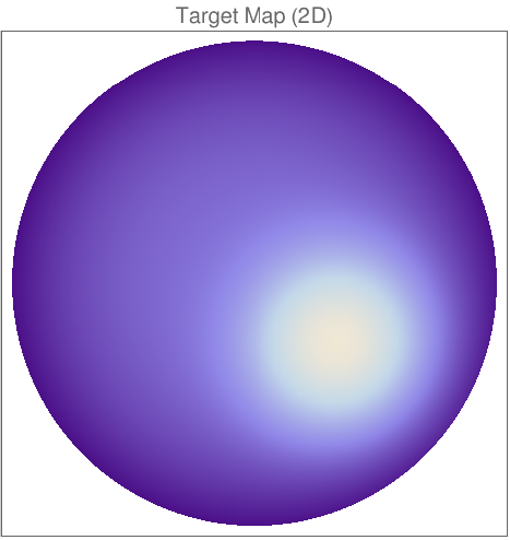
In introductory textbooks, least squares problems typically involve smooth, symmetric functions with clean, closed-form analytic solutions. However, in physical applications—such as localized atmospheric thermal turbulence or complex structural lens defects—the target function is often highly non-linear, off-center, and analytically non-integrable. In these cases, numerical computer calculations are strictly essential to evaluate the generalized Fourier coefficients.
Let us consider an asymmetrical, off-center thermal bloom pocket modeled as a localized Gaussian anomaly superimposed on a radial cubic deformation over the unit circular aperture: \[ f(r, \theta) = 3.5 \exp\left\{ -8 \left[ (r\cos\theta - 0.35)^2 + (r\sin\theta + 0.25)^2 \right] \right\} - 1.2r^3 . \]
Because of the shifted coordinates inside the exponential term, computing the projection inner product integrals \(\langle f, Z_n^{\pm m} \rangle\) analytically is impossible. We must deploy 2D numerical quadrature (numerical integration) to extract the best approximation coefficients in the mean-square sense.
Mathematica 14 Simulation & Optimization Script
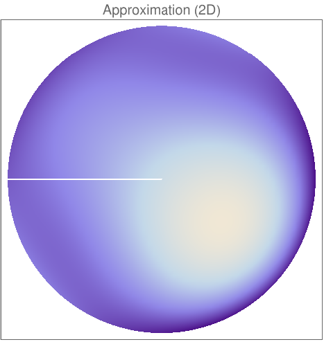
You can execute the following complete, self-contained Mathematica 14 script to numerically compute the generalized Fourier-Zernike coefficients up to radial degree \(N=4\) via adaptive 2D quadrature and visualize the structural minimization of the mean square deviation.
|
|
Pedagogical Elements:
-
The Role of the Jacobian Coordinate Weight: Inside the
NIntegrate[]function loop, the expression explicitly contains* rmatching the polar element metric rdr&thicksp;dθ. This demonstrates how polar space inherently alters the internal geometric weight density. -
Mean Convergence vs. Local Over-smoothing: Students will observe in the generated
errorPlotthat while global least-squares error metrics approach zero, localized spike errors persist near the coordinate point \((0.35, -0.25)\). Truncating at low radial frequencies (\(N=4\)) naturally smooths out steep structural gradients, highlighting why higher modal bounds are required to capture point-wise spatial variations.
Bessel's Inequality
Named after the prominent German astronomer and mathematician Friedrich Wilhelm Bessel (1784–1846), the following fundamental inequality was first formulated in 1828 during his investigations into planetary perturbations and Keplerian orbital math.
While its technical definition can appear abstractly dry, its geometric meaning is beautifully simple: it represents the infinite-dimensional analogue of the Pythagorean theorem. Just as the sum of the squared projections of a 3D vector onto two axes cannot exceed the total square length of the vector itself, the total aggregate energy contained within a finite set of coordinate components can never break the absolute energy barrier of the original function. It guarantees that our series approximations remain physically stable and bounded.
Theorem 1(Bessel's Inequality): Let ℌ be an inner product space or Hilbert space, and let { e₁, e₂, … , eₙ, …} be a given orthonormal sequence. Then for any element f from ℌ, Bessel's inequality states:
where ⟨· , ·⟩ denotes the standard inner product in the space.
By leveraging the sesquilinear properties of the inner product space, this expands into:
Since our basis sequence is strictly orthonormal, the cross-product components collapse under the Kronecker delta property ⟨ eₖ , e𝓂 ⟩ = δk,m. Substituting \(c_k = \langle \mathbf{e}_k, f \rangle\) and \(\overline{c_j} = \langle f, \mathbf{e}_j \rangle\), the relationship simplifies directly to:
Rearranging the remaining elements yields the inequality for any finite index bound \(n\):
Since this bounding upper constraint holds true for every finite \(n\), taking the limit as n → ∞ successfully establishes Bessel's global inequality statement.
Corollary 1 (Classical Trigonometric framework):
Then the corresponding bounding total energy relationship satisfies:
where \(E[f]\) represents the global structural energy of the \(2\ell\)-periodic function.
Example 5:
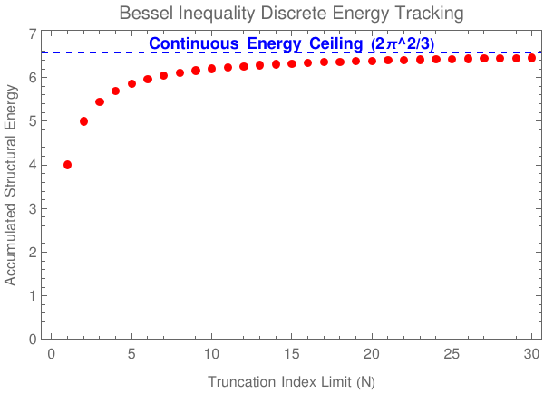
To demonstrate Bessel's inequality to students dynamically, we choose a classic piecewise discontinuous sawtooth wave \(f(x) = x\) over the periodic bounds \([-\pi, \pi]\) with a system scale \(\ell = \pi\). The global energy integral evaluates explicitly as: \[ E[f] = \frac{1}{\pi} \int_{-\pi}^{\pi} x^2 \,{\text d}x = \frac{2\pi^2}{3} \approx 6.57973 \]
Because our function is strictly an odd function, the cosine components vanish instantly (\(a_n = 0\)), while integrating the sine projections yields the sequence \(b_n = \frac{2(-1)^{n+1}}{n}\). Truncating our infinite summation to a restricted integer limit \(N\) changes the total energy identity into a strict unequal boundary: \[ \sum_{n=1}^N b_n^2 = \sum_{n=1}^N \frac{4}{n^2} < \frac{2\pi^2}{3} \]
You can execute the following code to numerically track how the sum of the projection squares steps up asymptotically toward the global energy ceiling without ever breaking it, proving Bessel's constraint visually:
Dense Sets, Completeness, and Bases
Recall that the closure \( \displaystyle \ \overline{A}\ \) of a subset A ⊆ ℌ is the smallest closed set containing A. It consists of all limits of convergent sequences (xₙ) where each xₙ ∈ A.
In other words, a subset A ⊆ ℌ is dense in a Hilbert space ℌ if for every f ∈ ℌ and every ε > 0, there exists g ∈ A with
=====================================================
A subset S ⊂ ℌ
is complete (or total) if its linear span is dense in ℌ. That is,\( \quad \overline{\mbox{span}(S)} = ℌ. \quad \) Alternatively, by the projection theorem, S
is complete if and only if the only vector orthogonal to all vectors in
is the zero vector (S⊥ = {0}).
Every dense set is a complete set. However, a complete set is generally NOT a dense set: A complete set only needs its linear combinations (finite sums, scaling, and their limits) to fill the space. The set of points themselves can be incredibly sparse, isolated, or discrete.
A Hilbert space is separable if and only if it contains a countable dense subset. Interestingly, this is perfectly mirrored by completeness: a Hilbert space is separable if and only if it possesses a countable complete orthonormal set (a Hilbert basis). While the dense subset itself must contain uncountably many points to cover every single neighborhood, the complete basis only needs countably many points because the vector addition and scalar multiplication do the heavy lifting of mapping out the rest of the space.
';The orthogonal expansion \( \displaystyle f(x) \sim \sum_{n\ge 0} c_n f_n (x) \) for a complete orthogonal system on [𝑎, b], holds in 𝔏² sense, but not necessarily pointwise, i.e. for a fixed x∈[𝑎, b] the series on the right hand side might not necessarily converge and, even if it does, it might not converge to f(x).
The Parseval Identity (Generalized)
Orthogonal Expansions
With the geometric framework of completeness and the Parseval identity established, we now possess the mathematical authorization to write down the generalized formula for reconstructing an arbitrary function \(f(x)\). Whether our chosen system yields trigonometric functions, Bessel functions, or classical orthogonal polynomials, the underlying algebraic engine remains identical.
If \(\{\phi_n(x)\}_{n=0}^{\infty}\) constitutes a complete orthogonal system in the weighted Hilbert space \(L^2([a,b], w(x)\text{d}x)\), any suitable function can be uniquely expanded using its generalized Fourier coefficients:
This elegant equation unifies several major classical expansions that appear across mathematical physics:
- Trigonometric Fourier Series: Arising from constant coefficients and periodic or Dirichlet boundary conditions.
- Bessel Series: Generated when solving problems in cylindrical coordinates where the weight function is \(w(x) = x\).
- Orthogonal Polynomials: Such as Legendre, Hermite, or Chebyshev systems, arising from unbounded intervals or singular boundary coordinates.
However, expressing an equality with an infinite sum of functions introduces a major topological hurdle. To safely manipulate these series in physical applications, we must answer a critical question: In what structural sense does this infinite sequence of graphs actually merge into our target function? To resolve this, we must examine the distinct Modes of Convergence.
Convergence
========================================================================== Note:Formula \eqref{EqOrtho.7} for the Fourier coefficients can be derived directly if the series \( \displaystyle \sum_{k\ge 0} c_k \phi_k (x) \) converges to f(x) uniformly. If this would be true, we could multiply the series by ϕn(x) ρ(x) and integrate from 0 to ℓ term by term. Because of orthogonality, all the integrals are zero except for k = n. Hence
Dense sets & Completeness
The (topological) closure of dense set A is all of ℌ; finite linear combinations from A can approximate any vector.
It should be emphasized that “Dense” means every function can be approximated arbitrarily well by finite expansions in the given system. This is the analytic expression of the geometric idea that dense set A “fills” the space: no nonzero vector is orthogonal to all of A.
In the Hilbert space 𝔏²([0,2π]) with inner product
Example 5: Consider the collection of cosine functions { 1, cos(x), cos(2x), cos(3x), … } on an interval of length 2π, which we know from the previous sections is orthogonal. We have
The term "complete" was introduced in 1910 by the Russian mathematician Vladimir Andreevich Steklov (1864--1926), a student of Alexander Lyapunov.
Example 6: Considered previously the collection of cosine functions { 1, cos(x), cos(2x), cos(3x), … } on an interval of length 2π in not complete, but it is orthogonal. Indeed, if f is any odd function (for instance, x or sinx), then \( \displaystyle f(-x) = -f(x) . \) Calculations show that \( \langle f, \cos (kx) \rangle =0 \) because the product of odd function and an even function is an odd function. ■ ■
A subset A ⊂ ℌ of a Hilbert space ℌ
is dense if its closure is the entire space \( \displaystyle
\quad \left( \overline{A} = ℌ \right) \quad \) . This means that every element in the Hilbert space can be approximated arbitrarily close by elements from A.
A subset S ⊂ ℌ
is complete (or total) if its linear span is dense in ℌ. That is,\( \quad \overline{\mbox{span}(S)} = ℌ. \quad \) Alternatively, by the projection theorem, S
is complete if and only if the only vector orthogonal to all vectors in
is the zero vector (S⊥ = {0}).
Every dense set is a complete set. However, a complete set is generally NOT a dense set: A complete set only needs its linear combinations (finite sums, scaling, and their limits) to fill the space. The set of points themselves can be incredibly sparse, isolated, or discrete.
A Hilbert space is separable if and only if it contains a countable dense subset. Interestingly, this is perfectly mirrored by completeness: a Hilbert space is separable if and only if it possesses a countable complete orthonormal set (a Hilbert basis). While the dense subset itself must contain uncountably many points to cover every single neighborhood, the complete basis only needs countably many points because the vector addition and scalar multiplication do the heavy lifting of mapping out the rest of the space.
';The orthogonal expansion \( \displaystyle f(x) \sim \sum_{n\ge 0} c_n f_n (x) \) for a complete orthogonal system on [𝑎, b], holds in 𝔏² sense, but not necessarily pointwise, i.e. for a fixed x∈[𝑎, b] the series on the right hand side might not necessarily converge and, even if it does, it might not converge to f(x).
Example 7: Considered previously the collection of cosine functions { 1, cos(x), cos(2x), cos(3x), … } on an interval of length 2π in not complete, but it is orthogonal. Indeed, if f is any odd function (for instance, x or sinx), then \( \displaystyle f(-x) = -f(x) . \) Calculations show that \( \langle f, \cos (kx) \rangle =0 \) because the product of odd function and an even function is an odd function. ■ ■
Example 8: There are known other orthogonal and complete sets of functions that are used in other than differential equations areas. In particular, Li--Torney system of step function is very useful in computer science. The collection of Walsh functions form a complete orthogonal set of functions that can be used to represent any discrete function---just like trigonometric functions can be used to represent any continuous function in Fourier analysis. These functions as well as the Walsh--Hadamard code are named after the American mathematician Joseph L. Walsh (1895--1973). Applications of the Walsh functions can be found wherever digit representations are used, including speech recognition, medical and biological image processing, and digital holography. The Haar wavelet is a sequence of rescaled "square-shaped" functions which together form a wavelet family or basis. Wavelet analysis is similar to Fourier analysis. The Haar sequence was proposed in 1909 by the Hungarian mathematician Alfréd Haar (1885--1933).
The Faber–Schauder system is a Schauder basis for the space ℭ([0, 1]) of continuous functions on [0, 1]. The Franklin system is obtained from the Faber--Schauder system by the Gram–Schmidt orthonormalization procedure.
■The Parseval identity
Parseval's identity holds if and only if
Example 9: Expand the function
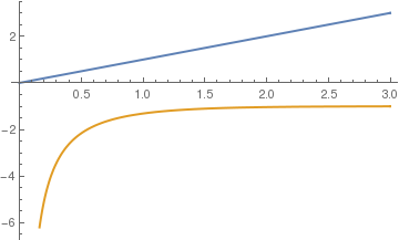
The solution of the differential equation \( y'' + \lambda\,y =0 \) may have one of three forms, depending on λ, so it is necessary to consider these cases. Let us start with λ = 0, the general solution becomes a linear function
If λ is negative, we can let λ = -μ² so that μ > 0. Then the differential equation for y becomes
Next consider λ > 0, then the general solution is
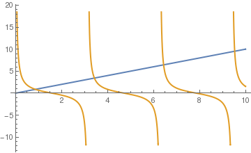
To find the expansion for f in terms of the eigenfunctions, we write
Where Do Orthogonal Functions Come From?
The first thing to be looked at is the Gram-Schmidt process.
=================================================
Orthogonal Expansions
There are significant differences between the behavior of Fourier- and power-series expansions. A power series is essentially an expansion about a point, using only information from that point about the function to be expanded (including, of course, the values of its derivatives). We already know that such expansions only converge within a radius of convergence defined by the position of the nearest singularity. However, a Fourier series (or any expansion in orthogonal functions) uses information from the entire expansion interval, and therefore can describe functions that have “nonpathological” singularities within that interval. However, we also know that the representation of a function by an orthogonal expansion is only guaranteed to converge in the mean. This feature comes into play for the expansion of functions with discontinuities, where there is no unique value to which the expansion must converge. However, for Fourier series, it can be shown that if a function f(x) satisfying the Dirichlet conditions is discontinuous at a point x0, its Fourier series evaluated at that point will be the arithmetic average of the limits of the left and right approaches.
Riemann--Lebesgue Lemma
Bessel's inequality shows that for any square integrable function f ∈ 𝔏²([0, ℓ], ρ), the series
Convergence
Formula \eqref{EqOrtho.7} tells us that there is a mapping
It is most natural to consider pointwise convergence, where we examine the discrepancy at every point. It is difficult (may be impossible) to provide general results about pointwise convergence for general orthogonal functions, but for Fourier series a lot has been done. We have to ask that f(x) be a lot smoother than just belonging to 𝔏², which is a "big" space of functions. You might think having f(x) continuous would be enough, but that obviously does not work at Gibbs phenomenon shows. Here is a slightly different statement of the conditions copied from Keener:
If function f(x) has continuous first derivatives on the interval, except possibly at a finite number of points at which there is a jump in f(x), where left and right derivatives must exist. Then the Fourier series of f converges to ½(f(x+)+f(x−)) for every point in the open interval (0,ℓ). At x=0 and ℓ, the series converges to ½(f(0+)+f(ℓ−)).
The most remarkable result regarding pointwise convergence almost everywhere was obtained by Hans Rademacher (1922) and Dmitrii Menshov (1923).
Another form of convergence is uniform convergence. This used to be the gold standard of convergence. For continuous functions, you can measure the maximum difference between the series and the function written:
- Bari, N.K.,
- Huaien Li and David C. Torney, A complete system of orthogonal step functions, Proceedings of the American Mathematical Society, 132, No 12, 2004, pp. 3491--3502.
- Menchoff, D.E., (1923), "Sur les séries de fonctions orthogonales. (Première Partie. La convergence.).", Fundamenta Mathematicae (in French), 4: 82–105, doi:10.4064/fm-4-1-82-105
- Rademacher, Hans (1922), "Einige Sätze über Reihen von allgemeinen Orthogonalfunktionen", Mathematische Annalen, Springer Berlin / Heidelberg, 87: 112–138, doi:10.1007/BF01458040
- Sturm–Liouville problem.
- Titchmarsh, E.C., Eigenfunction Expansions Associated with Second-order Differential Equations. Part I (1946); 2nd. edition (1962).
- Titchmarsh, E.C., Eigenfunction Expansions Associated with Second-order Differential Equations. Part II (1958).
- J. L. Walsh, A closed set of normal orthogonal functions, American Journal of Mathematics, 45, (1923), 5--24.
Return to Mathematica page
Return to the main page (APMA0340)
Return to the Part 1 Matrix Algebra
Return to the Part 2 Linear Systems of Ordinary Differential Equations
Return to the Part 3 Non-linear Systems of Ordinary Differential Equations
Return to the Part 4 Numerical Methods
Return to the Part 5 Fourier Series
Return to the Part 6 Partial Differential Equations
Return to the Part 7 Special Functions