This tutorial was made solely for the purpose of education and it was designed
for students taking Applied Math 0340. It is primarily for students who
have some experience using Mathematica. If you have never used
Mathematica before and would like to learn more of the basics for this computer algebra system, it is strongly recommended looking at the APMA
0330 tutorial. As a friendly reminder, don't forget to clear variables in use and/or the kernel. The Mathematica commands in this tutorial are all written in bold black font, while Mathematica output is in regular fonts.
Finally, you can copy and paste all commands into your Mathematica notebook, change the parameters, and run them because the tutorial is under the terms of the GNU General Public License
(GPL). You, as the user, are free to use the scripts for your needs to learn the Mathematica program, and have
the right to distribute and refer to this tutorial, as long as
this tutorial is accredited appropriately. The tutorial accompanies the
textbookApplied Differential Equations.
The Primary Course by Vladimir Dobrushkin, CRC Press, 2015; http://www.crcpress.com/product/isbn/9781439851043
Return to computing page for the first course APMA0330
Return to computing page for the second course APMA0340
Return to Mathematica tutorial for the first course APMA0330
Return to Mathematica tutorial for the second course APMA0340
Return to the main page for the
first course APMA0330
Return to the main page for the
second course APMA0340
Return to Part VI of the course APMA0340
Introduction to Linear Algebra
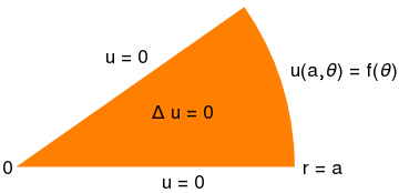
To solve the given boundary value problem, we apply separation of variables. So
we seek partial nontrivial (not identically zero) solutions of the auxiliary
problem
Note that λ = 0 is not an eigenvalue because the corresponding
eigenfunction Θ0 = a+ bθ must be identically zero to
satisfy the homogeneous boundary condition.
Therefore, we get a discrete sequence of positive eigenvalues
\[
u(x,y) = \frac{2}{\pi} \int_0^{\infty} u^s (x, k)\,\sin (ky)\,{\text d}k = \frac{1}{\pi}\,\int_{-\infty}^{+\infty} \frac{y}{(x-\xi )^2 + y^2} \,f(\xi )\,{\text d}\xi . .
\]
The Green function for this Dirichlet problem for Laplace's equation in the upper half-plane is known as the Poisson kernel:
\[
P(x,y) = \frac{1}{\pi}\cdot \frac{y}{x^2 + y^2} \quad \Longrightarrow \quad u(x,y) = \int_{-\infty}^{\infty} P(x-\xi , y)\,f(\xi )\,{\text d}\xi .
\]
Example A (temperature distribution):
Suppose the temperature along the real axis is maintained at
T = 1 for −1 ≤ ξ ≤ 1 and T = 0 everywhere else on the real axis. We can
use the Poisson kernel to find the temperature everywhere on the upper half-plane. We have
\[
u(x,y) = \frac{y}{\pi} \int_{-1}^1 \frac{{\text d}\xi}{(x-\xi )^2 + y^2} .
\]
The integral can be done by substitution, though Mathematica helps
Example 4:
Let us consider the Neumann problem for Laplace's 2D equation
\[
\begin{split}
\nabla^2 u &= 0 , \quad y > 0,
\\
\left. \frac{\partial u}{\partial \hat{\bf n}} \right\vert_{y=0} &= - \frac{\partial u}{\partial y}(x, 0) = g(x) , \quad x\in \mathbb{R} ,
\\
u , \ u_x , \ u_y \to 0& \quad \mbox{as} \quad x \to \pm \infty , \ y \to +\infty ;
\\
\int_{-\infty}^{+\infty} g(x)\,{\text d}x &= 0 \qquad (\mbox{compatibility condition}).
\end{split}
\]
The Neumann problem may have a solution when the compatibility condition is not valid---in this case, the solution will not stay bounded as y → +∞. We require this condition holds because we will apply Fourier transformation to the Neuman problem, and zero Fourier mode forces \( \displaystyle \quad \hat{g} (0) = \int_{\mathbb{R}} g(x)\,{\text d}x = 0 . \)
To solve this boundary value problem, we apply cosine-Fourier transform with respect to variable y. Integrating by parts twice and taking into account the regularity condition at infinity, we get
\begin{align*}
\int_0^{\infty} \frac{\partial^2 u}{\partial y^2}\,\cos (ky)\,{\text d}y &= \left. \frac{\partial u}{\partial y}\,\cos (ky) \right\vert_{y=0}^{\infty} + k \int_0^{\infty}
\frac{\partial u}{\partial y} \,\sin (ky)\,{\text d}y
\\
&= g(x) + k \,\left. u(x,y)\,\sin (ky) \right\vert_{y=0}^{\infty} - k^2 \int_0^{\infty} u(x,y)\,\cos (ky)\,{\text d}y
\\
&= g(x) - k^2 u^c (x,k) ,
\end{align*}
where
\[
u^c (x,k) = \int_0^{\infty} u(x,y)\,\cos (ky)\,{\text d} y
\]
is the cosine Fourier transform of unknown function u. This leads to the ODE in variable x ∈ ℝ:
\[
\frac{{\text d}^2 u^c}{{\text d} x^2} - k^2 u^c + g(x) = 0 , \qquad x\in \mathbb{R} .
\]
We ask Mathematica to solve this ODE:
Finally, we integrate this expression and obtain
\[
u(x,y) = \frac{1}{2\pi}\,\int_x^{\infty} \ln \left( (x-\xi )^2 + y^2 \right) g(\xi )\,{\text d}\xi - \frac{1}{2\pi}\,\int_{-\infty}^x \ln \left( (x-\xi )^2 + y^2 \right) g(\xi )\,{\text d}\xi + C ,
\tag{4.2}
\]
Integrate[a/(a^2 + y^2), a]
1/2 Log[a^2 + y^2]
where C is a constant of integration. As formula (4.2) shows, the Neumann problem has a solution up to arbitrary additive constant. We demonstrate solutions of the Neumann problem in a couple of numerical examples.
Example A (compatibility condition fails):
We work in the upper half-plane
\[
\mathbb{H} = \left\{ (x,y) \in \mathbb{R}^2 \ : \ y > 0 \right\} ,
\]
with Neumann condition
\[
\frac{\partial u}{\partial y}(x,0) = -g(x) .
\]
Let us take u(x, y) = xy. This function is harmonic because
\[
\frac{\partial^2}{\partial x^2}\,u(x,y) = \frac{\partial^2}{\partial y^2}\,u(x,y) = 0.
\]
The Neuman boundary condition prescribes normal derivative, not the value of the function, so it reads
\[
\left. \frac{\partial u}{\partial y} \right\vert_{y=0} = x \ \nexists \ 𝔏²(\mathbb{R}) .
\]
Formally, function uy(x,0) = x is not integrable; however, under the Cauchy principal value regularization, the compatibility condition holds:
\[
\mbox{V.P.} \int_{-\infty}^{\infty} x\,{\text d}x = \lim_{R\to +\infty} \int_{-R}^R x\,{\text d}x = 0.
\]
On the boundary y = 0, the outward unit normal is n = (0,-1), so
\[
\frac{\partial u}{\partial {\bf n}} = \nabla u\bullet \mathbf{n} =(u_x, u_y)\bullet (0,-1) = -u_y .
\]
Since uy(x,y) = x, we get on y = 0:
\[
\frac{\partial u}{\partial {\bf n}}(x,0)=-x.
\]
So u(x,y) = xy solves the Neumann problem.
A standard trick is to write the kernel as the real part of a complex Cauchy kernel:
\[
\frac{x-\xi}{(x-\xi )^2+y^2}=\Re \left( \frac{1}{x-\xi +{\bf j}y}\right) .
\]
So
\[
\int _{-\infty }^{\infty }\frac{|x-\xi |}{(x-\xi )^2+y^2}\, e^{-\xi ^2}\, d\xi = \Re \left( \int _{-\infty }^{\infty }\frac{e^{-\xi ^2}}{x-\xi +{\bf j}y}\, d\xi \right) .
\]
Introduce the complex variable z = x + ⅉy.
A classical Gaussian integral identity is:
\[
\int _{-\infty }^{\infty }\frac{e^{-\xi ^2}}{z-\xi }\, d\xi =\pi {\bf j}\, e^{-z^2}\, \operatorname{erfc} (-{\bf j}z),
\]
and differentiating with respect to z gives an identity for
\( \displaystyle \quad \int \frac{\xi e^{-\xi ^2}}{z-\xi }\, d\xi . \quad \)
Carrying out the differentiation and simplification yields the closed form:
\[
I(x,y)=\int _{-\infty }^{\infty }\frac{y}{(x-\xi )^2+y^2}\, 2\xi e^{-\xi ^2}\, d\xi =
\pi \, e^{-x^2-y^2}\left[ \operatorname{erf} (x+iy)+\operatorname{erf} (x-iy)\right] .
\]
Thus, the solution is:
\[
u(x,y)=C+\frac{1}{\pi }I(x,y)=C+e^{-x^2-y^2}\left[ \operatorname{erf} (x+{\bf j}y)+\operatorname{erf} (x-{\bf j}y)\right] .
\]
This is a real‑valued function because the two terms are complex conjugates.
This is the wedge analogue of the Poisson kernel for the disk/half-plane.
Example 5:
Let the wedge be
\[
W_{\alpha }=\{ (r,\theta ):r>0,\; 0<\theta <\alpha \} .
\tag{2.1}
\]
We are looking for a harmonic function u(r, θ) in this infinite wedge domain satisfying the Dirichlet boundary conditions:
\[
u(r, 0) = f_0 (r) , \qquad u(r, \alpha ) = f_{\alpha} (r) .
\tag{2.2}
\]
We map the wedge to upper half-plane
\[
w = z^{\pi /\alpha },\quad z=r\,e^{{\bf j}\theta } ,
\tag{2.3}
\]
where z = x + ⅉy and j = ⅉ is the imahinary unit on the complex plane ℂ, so ⅉ² = −1.
As θ runs from 0 to α, the argument of w runs from 0 to π, so Wα maps onto the upper half-plane
\[
\mathbb{H}= \{ w=x+{\bf j}\,y \ : \ y>0\} .
\]
Pull back to the wedge.
Let u(r, θ) be harmonic in Wα with boundary data f prescribed on the rays . Under the map w = zπ/α, the boundary of the wedge corresponds to the real axis, but the boundary parameterization changes.
Write
\[
w=r^{\pi /\alpha }e^{i\pi \theta /\alpha }=x+{\bf j}y.
\]
On the boundary, θ = 0 or θ = α, w is real and nonzero. A convenient way to encode the boundary data is to think of f as a function of the argument ϕ ∈ (0, α) along the circular arc at some fixed radius, then use separation of variables. That route leads more cleanly to the standard closed form, so let’s switch to that.
\[
P_{\alpha }(r,\theta ;\phi )=\frac{1}{\alpha }\frac{\sinh \! \left( \frac{\pi }{\alpha }\ln r\right) }{\cosh \! \left( \frac{\pi }{\alpha }\ln r\right) -\cos \! \left( \frac{\pi }{\alpha }(\theta -\phi )\right) } ,
\]
and the harmonic extension is
\[
u(r,\theta )=\int _0^{\alpha }P_{\alpha }(r,\theta ;\phi )\, f(\phi )\, d\phi .
\]
■
End of Example 5
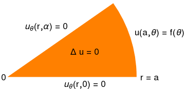
Example 6:
We seek a harmonic function u(r, θ) in the wedge domain Wα = { (r, θ) : 0 < r < ∞, 0 < θ < α } satisfying Neuman data of the sides
\[
\frac{\partial u}{\partial n} \left( r, 0 \right) = g_0 (r) , \qquad \frac{\partial u}{\partial n} \left( r, \alpha \right) = g_{\alpha} (r) , \qquad r > 0 .
\]
Outward normals on the sides give
\[
\frac{\partial u}{\partial n} \left( r, 0 \right) = - \frac{1}{r} \,\frac{\partial u}{\partial \theta} \left( r, 0 \right) = g_0 (r) , \qquad \frac{\partial u}{\partial n} \left( r, \alpha \right) = \frac{1}{r} \,\frac{\partial u}{\partial \theta} \left( r, \alpha \right) = g_{\alpha} (r) .
\]
So
\[
u_{\theta} (r, 0) = -r\,g_0 (r) , \qquad u_{\theta} (r, \alpha ) = r\,g_\alpha (r) .
\]
Its solution is determined up to an additive constant:
\[
u(r, \theta ) = C + \int_0^{\infty} N_0 (r, \theta ; \rho )\,g_0 (\rho )\,\rho\,{\text d}\rho + \int_0^{\infty} N_{\alpha} (r, \theta ; \rho )\,g_{\alpha} (\rho )\,\rho\,{\text d}\rho ,
\]
where N₁ and Nα are the Neumann Poisson kernels associated with the sides. They are normal derivatives (in source variable) of the Neumann Green function G for the wedge
Map the wedge to the upper half-plane vis
\[
w = z^{\pi /\alpha} , \quad z = r\,e^{{\bf j}\theta} \qquad \Longrightarrow \qquad w = r^{\pi /\alpha}e^{{\bf j}\theta\pi /\alpha} .
\]
Write
\[
X = r^{\pi /\alpha} \cos\frac{\pi\theta}{\alpha} , \quad Y = r^{\pi /\alpha} \sin\frac{\pi\theta}{\alpha} , \quad \xi (\rho , \phi ) = \rho^{\pi /\alpha} \cos \frac{\pi\phi}{\alpha} .
\]
The Neumann Poisson kernel for the upper half-plane (data on real axis) is
\[
P_N (X, Y; \xi ) = \frac{1}{\pi} \left[ \frac{Y}{(X- \xi )^2 + Y^2} + \frac{Y}{(X+ \xi )^2 + Y^2} \right] .
\]
■
End of Example 6
Explicit Green Function for a Wedge.
For the wedge Wα, the Green function is:
Example 7:
The Green function for Laplace's equation in ℝ² is a solution (in distributions) of the following problem
\[
\Delta G(x, y) = \delta (x)\,\delta (y) \qquad \iff \qquad \frac{\partial^2 G}{\partial x^2} + \frac{\partial^2 G}{\partial y^2} = \delta (x)\,\delta (y) ,
\tag{4.1}
\]
where δ is the Dirac delta function. Then Poisson's equation
\[
\Delta u = f
\]
has the solution expressed via the Green function
\[
u(x,y) = \iint_{\mathbb{R}^2} G(x-\xi , y-\eta )\,f(\xi , \eta )\,{\text d}\xi\,{\text d}\eta .
\]
Application of double Fourier transform to Eq.(4.1) yields the algebraic equation
\[
- \left( \xi^2 + \eta^2 \right) G^{FF} = 1 ,
\]
where GFF is the double Fourier transform of the Green function. Using the inverse Fourier transform, we find
\[
G(x,y) = \frac{1}{\pi^2} \int_{-\infty}^{\infty} {\text d}\xi \int_{-\infty}^{\infty} {\text d}\eta\, e^{{\bf j}x\xi + {\bf j}y\eta}
\]
Mathematica helps:
So we have
\[
G(x,y) = \frac{1}{2\pi}\,\ln \sqrt{x^2 + y^2} = \frac{1}{4\pi}\,\ln \left( x^2 + y^2 \right) .
\tag{4.2}
\]
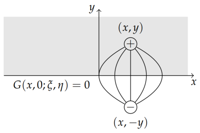
Next, we find the Green’s function for the half plane, { (x, y) : y > 0 }, using the Method of Images.
This problem can be solved using the result for the Green’s function for the infinite plane. We use the Method of Images to construct a function such that G = 0
on the boundary, y = 0. Namely, we use the image of the point (x, y)
with respect to the
x-axis, (x, −y).
Imagine that the Green’s function G(x, y, ξ, η) = G(x −ξ, y −η)
represents a point charge at (x, y)
and G(x, y, ξ, η)
provides the electric potential, or response, at (ξ, η). This single charge cannot yield a zero potential along the x-axis (y = 0). One needs an additional charge to yield a zero equipotential line. This is shown in Figure 4.1.
Figure 4,1: The source and image source for the Green’s function.
The positive charge has a source of \( \displaystyle \quad \delta (\mathbf{r} - \mathbf{r}' ) \quad \)
at r = (x, y)
and the negative charge is represented by the source\( \displaystyle \quad \delta (\mathbf{r}^{\ast} - \mathbf{r}' ) \quad \)
at r✶ = (x, −y). We construct the Green’s functions at these two points and introduce a negative sign for the negative image source. Thus, we have
\[
G(x, y,\xi, \eta ) = \frac{1}{4\pi}\,\ln \left( (x-\xi )^2 + (y-\eta )^2 \right) - \frac{1}{4\pi}\,\ln \left( (x-\xi )^2 + (y+\eta )^2 \right) .
\]
These functions satisfy the differential equation ΔG = δ;(x −ξ) δ;(y −η) and the boundary condition G(x, 0) = 0.
■
End of Example 7
Special Explicit Solutions for Common Boundary Data
(a) Constant on one boundary, zero on the other.
Solve:
\[
u(r,0)=0,\qquad u(r,\alpha )=1.
\]
Solution:
\[
u(r,\theta )=\frac{\theta }{\alpha }.
\]
(This is harmonic because it is independent of r.)
This appears in Sneddon’s treatment of mixed problems.
Shapiro–Lopatinskiĭ condition
The
Shapiro–Lopatinskiĭ condition (or Lopatinskiĭ-Shapiro condition) is a fundamental criterion in the theory of linear partial differential equations that ensures the Fredholm solvability of boundary value problems (BVPs) for elliptic operators. It requires that boundary operators are independent modulo the factor
(roots in the lower half-plane) of the operator's polynomial symbo
We present this condition in a simple version used in elliptic boundary value theory (Agmon–Douglis–Nirenberg, Lions–Magenes, Kozlov–Maz’ya–Rossmann).
Let us consider Laplace's equation Δu = 0 in some domain Ω with smooth boundary ∂Ω subject to the boundary condition
\[
Bu = b_1(x)\, \partial _n u +b_2(x)\, \partial _{\tau }u+b_3(x)\, u\quad \mathrm{on\ }\partial \Omega .
\]
Here
n = outward normal vector of unit length,
τ is a unit vector in tangent direction.
The Shapiro–Lopatinskiĭ condition is a local condition at each boundary point.
At a boundary point, flatten the boundary so that locally:
boundary = { x₂ = 0 },
domain = { x₂ > 0}
normal = e₂,
tangential direction = e₁.
Freeze coefficients at the boundary point.
Take the tangential Fourier transform in x₁:
\[
u(x_1,x_2)=e^{{\bf j}\xi x_1}v(x_2).
\]
Then the PDE becomes an ODE:
\[
v''(x_2)-\xi ^2v(x_2)=0.
\]
The decaying solution in the half-plane x₂ > 0 is
\[
v(x_2 ) = C\,e^{-|\xi |x_2}.
\]
Apply the boundary operator to this decaying solution:
we get the boundary symbol = -b₁| ξ | + ⅉ b₂ξ + b₃.
The principal part ignores the lower‑order term b₃u as
of lower order, so the principal boundary symbol is
Neumann: ∂nu = 0 ⇒ b₁ = 1, b₂ = b₃ = 0
b(ξ) = -|ξ| ≠ 0 for ξ ≠ 0 ⇒ SL holds (the issue is the usual “constant ambiguity”).
Pure tangential: ∂τu = 0 ⇒ b₂ = 1, b₁ = b₃ = 0,
b(ξ) = ⅉξ ≠ 0 for ξ ≠ 0 ⇒ SL holds (but this is not a good physical boundary condition for Laplace equation).
Shapiro–Lopatinskiĭ condition (for Laplace in 2D) says:
For every real ξ ≠ 0, the boundary symbol must not vanish:
Analytic functions
Analytic functions
Recall that both the real and imaginary parts of an analytic function satisfy
Laplace’s equation in two dimensions. Suppose the region of interest is
defined by the angular wedge W = 0 ≤ θ ≤ α. Consider the
analytic function
of which we consider the principal branch. If α = π/m for some
integer m, then f(z) is analytic everywhere. If
α is an arbitrary real number, then f(z) may
have a branch point at the origin, but we may choose the branch cut so that
f(z) is still analytic in our region everywhere except at the
origin. In fact the function \( f_n (z) =
z^{n\pi /\alpha} \) for any integer n has the
same nice properties. Then its real part \(
u(r, \theta ) = \Re f(z) = r^{\pi /\alpha} \cos \frac{\pi\theta}{\alpha} \)
and imaginary part \(
v(t, \theta ) = \Im f(z) = r^{\pi /\alpha} \sin \frac{\pi\theta}{\alpha} \)
are both solutions of the Laplace's equation:
\[
\Delta u =0 \qquad\mbox{and}\qquad \Delta v =0
\]
in the wedge. Thus, the potential in a wedge-shaped region W with
opening angle α and conducting boundaries at potential V0
is described by the complex potential
The coefficients an must be chosen to
satisfy any remaining boundary conditions in r.
Since the origin is included within our wedge-shaped region W, the sum
is over positive n only, so that the potential remains finite. Then the
potential near the origin (small r) is dominated by the first (n
= 1) term,and the field near the origin has components:
This is true only when \( -1 + \frac{\pi}{\alpha} > 0
\) Otherwise, π < α, the field is unbounded unless the
first coefficient is zero.
As one might expect, the behavior of solution near r = 0 has to be
restricted:
\[
v(r,\theta ) = c_0 + c_1 \ln r + o(1) \qquad\mbox{as} \quad r \to 0 ,
\]
where c0 and c1 are some constants. The
constant c0 cannot be chosen arbitrary. (It is analogous to
the so-called blockage coefficient in other potential flows.) The above
condition on behavior of harmonic function near the corner point is called the
wedge condition.
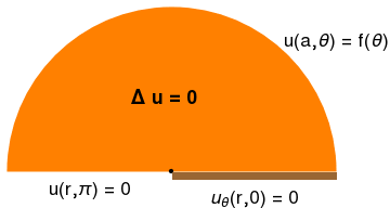
For instance, if we consider the Neumann boundary conditions on the two sides
of the wedge,
where f is a specified function. Evidently, the solution of the
problem, u, is not unique because we can always add
c0 + c1 log r, where
c0 and c1 are arbitrary constants.
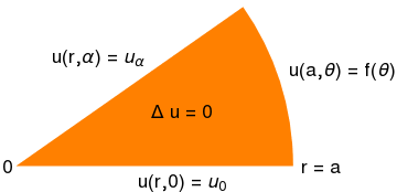
We reduce the given boundary value problem to the problem considered in the
previous example with homogeneous boundary conditions by representing the
unknown function u(r,θ) as a sum of two functions:
Actually, instead of w can be used any function that satisfies the
prescribed boundary conditions: \( w(r,0) = u_0 \)
and \( w(r,\alpha ) = u_{\alpha} . \) Then for
function v(r,θ) we get the following boundary value problem
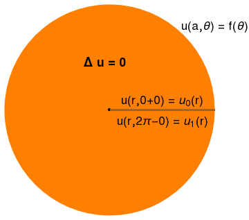
If the boundary conditions on the crack are the same, u0 =
u1, the solution can be obtained from our first two examples
by taking the limit \( \lim_{\alpha \to 2\pi} u(r, \theta ) . \) When they are not the same, the problem becomes very hard to solve.
■
End of Example 1
Copson, E.T., An Introduction to the Theory of Functions of a Complex Variable, Oxford University Press, London, 1935.
Kellogg, O.D., Foundations of potential theory, Dover Publications, 2010.
Sneddon, I.N., Mixed Boundary Value Problems in Potential Theory, North-Holland Publishing Company, 1966.
Return to the main page (APMA0340)
Return to the Part 1 Matrix Algebra
Return to the Part 2 Linear Systems of Ordinary Differential Equations
Return to the Part 3 Non-linear Systems of Ordinary Differential Equations
Return to the Part 4 Numerical Methods
Return to the Part 5 Fourier Series
Return to the Part 6 Partial Differential Equations
Return to the Part 7 Special Functions