Return to computing page for the first course APMA0330
Return to computing page for the second course APMA0340
Return to computing page for the fourth course APMA0360
Return to Mathematica tutorial for the first course APMA0330
Return to Mathematica tutorial for the second course APMA0340
Return to Mathematica tutorial for the fourth course APMA0360
Return to the main page for the course APMA0330
Return to the main page for the course APMA0340
Return to the main page for the course APMA0360
Introduction to Linear Algebra with Mathematica
Two functions f(x) and g(x) from Hilbert space 𝔏² are called orthogonal if their inner product—typically defined as the definite integral of their product over a specific interval
—equals zero, \( \displaystyle \quad \left( \left\langle f, g \right\rangle = \int_a^b f(x)^{\ast} g(x)\,{\text d} x = 0 \right) . \quad \) Here 𝑎 and b are some real numbers, possibly infinite, and \( \displaystyle \quad f(x)^{\ast} = \overline{f(x)} \quad \) is complex conjugate function to f(x).
Let f : [𝑎, b] → ℂ be a complex-valued function from some vector space X. A norm of function f, denoted as ∥f∥ is a function ∥·∥ : X → [0, ∞) that assigns a non-negative real number to a function f ∈ X, representing its length, magnitude, or size. It acts as a generalization of distance, satisfying properties of non-negativity, absolute scalability (∥k f∥ = |k| ∥f∥), and the triangle inequality (∥f + g∥ ≤ ∥f∥ + ∥g∥).
A
normalized function is a function whose norm (typically the 𝔏² norm) is exactly 1.
In this section, we mostly consider the Euclidean norm:
\[
\| f \| = + \left( \int_a^b |f(x)|\,{\text d} x \right)^{1/2} .
\]
A set {ω₁(x), ω₂(x), …} of linearly independent functions from 𝔏² is called orthonormal system if
every vector has a unit length (norm of 1) and all distinct vectors are mutually orthogonal (inner product is 0),
\[
\left\langle \omega_n , \omega_k \right\rangle = \begin{cases}
1, & \quad \mbox{if}\quad n=k ,
\\
0, & \quad \mbox{otherwise}.
\end{cases}
\]
A typical orthonormal system form functions
\[
\omega_n (x) = \frac{1}{\sqrt{\pi}}\,\sin (nx) , \qquad -\pi \le x \le \pi , \quad \forall n \in \mathbb{Z}.
\]
Let f ∈ 𝔏². Numbers 𝑎ₙ = ⟨f, ωₙ⟩ are called the Fourier coefficients of function f with respect to the orthonormal system { ωₙ }, and series \( \displaystyle \quad \sum_n a_n \omega_n (x) \quad \) is referred to as the Fourier series of function f. Its finite partial sum is
\[
S_N (f; x) = \sum_{n=1}^N a_n \omega_n (x) .
\]
Theorem 1 (Bessel inequality):
If function f ∈ 𝔏² and the set {ω₁(x), ω₂(x), …} forms an orthonormal system, then the Bessel inequality holds:
\[
\sum_{n=1}^{\infty} \left\vert a_n \right\vert^2 = \sum_{n=1}^{\infty} \left\vert \left\langle f, \omega_n \right\rangle \right\vert^2 \leqslant \| f \|^2 .
\]
Let us determine the norm of difference
\begin{align*}
0 &\le \| f(x) - S_n (f; x) \|^2 = \left\langle f(x) - S_n (f; x) , f(x) - S_n (f; x) \right\rangle
\\
&= \left\langle f, f \right\rangle - \left\langle f, S_n \right\rangle - \left\langle S_n , f \right\rangle + \left\langle S_n , S_n \right\rangle
\\
&= \| f \|^2 - \left\langle f, \sum_{k=1}^n a_k \omega_k \right\rangle - \left\langle \sum_{k=1}^n a_k \omega_k , f \right\rangle + \left\langle \sum_{k=1}^n a_k \omega_k , \sum_{k=1}^n a_k \omega_k \right\rangle
\\
&= \| f \|^2 - \sum_{k=1}^n a_k \left\langle f, \omega_k \right\rangle - \sum_{k=1}^n a_k^{\ast} \left\langle\omega_k , f\right\rangle + \sum_{k,i=1}^n a_i a_k^{\ast} \left\langle \omega_i , \omega_k \right\rangle
\\
&= \| f \|^2 - \sum_{k=1}^n \left\vert a_k \right\vert^2 .
\end{align*}
Therefore, we get the inequality
\[
\sum_{k=1}^n \left\vert a_k \right\vert^2 \leqslant \| f \|^2
\]
that is valid for any positive integer n. So application of limit when n → ∞ gives the Bessel inequality.
Example 1:
Consider the Hilbert space 𝔏²[-π , π]
with the standard inner product
\[
\langle f , g \rangle = \int_{-\pi}^{\pi} f(x)\,g(x)\,{\text d}x
\]
because it is a real vector space.
Take the orthonormal system
\[
\omega _1(x)=\frac{1}{\sqrt{2}},\qquad \omega _2(x)=\cos x,\qquad \omega _3(x)=\sin x.
\]
These are the first three functions of the Fourier orthonormal basis.
Let the function be
\[
f(x)=x.
\]
Step 1. Compute the Fourier coefficients 𝑎ₙ = ⟨ f , ωₙ ⟩.
Coefficient for ω₁(x) = 1/√2, we have
\[
a_1=\left< x,\frac{1}{\sqrt{2}}\right> =\frac{1}{\pi \sqrt{2}}\int _{-\pi }^{\pi }x\, dx=0
\]
because the integrand is odd.
Coefficient for ω₂(x) = cosx is
\[
a_2=\frac{1}{\pi }\int _{-\pi }^{\pi }x\cos x\, dx=0
\]
again odd integrand.
Coefficient for ω₃(x) = sinx becomes
\[
a_3=\frac{1}{\pi }\int _{-\pi }^{\pi }x\sin x\, dx.
\]
Here the integrand is even, so
\[
a_3=\frac{2}{\pi }\int _0^{\pi }x\sin x\, {\text d}x.
\]
Integrate by parts:
\[
\int _0^{\pi }x\sin x\, {\text d}x=\left[ -x\cos x\right] _0^{\pi }+\int _0^{\pi }\cos x\, {\text d}x=\pi +0=\pi .
\]
Thus,
\[
a_3 =\frac{2}{\pi }\cdot \pi =2.
\]
Integrate[x*Sin[x], {x, -Pi, Pi}]/Pi
2
So the first three coefficients are:
\[
a_1=0,\qquad a_2=0,\qquad a_3=2.
\]
Apply Bessel’s inequality
\[
\sum _{n=1}^{\infty }|a_n|^2\leq \| f\| ^2.
\]
Let’s compute both sides.
The left-hand side (partial sum) is
\[
|a_1|^2+|a_2|^2+|a_3|^2=0+0+4=4.
\]
the right-hand side: the norm of f(x) = x
\[
\| f\| ^2=\frac{1}{\pi }\int _{-\pi }^{\pi }x^2\, dx=\frac{2}{\pi }\int _0^{\pi }x^2\, dx=\frac{2}{\pi }\cdot \frac{\pi ^3}{3}=\frac{2\pi ^2}{3}.
\]
Since \( \displaystyle \quad \frac{2\pi ^2}{3}\approx 6.58, \quad \) we have
\[
4\leq \frac{2\pi ^2}{3},
\]
which confirms Bessel’s inequality.
What this example shows:
Even if we take only one nonzero coefficient (𝑎₃ = 2), the sum of squares
\[
|a_3|^2=4
\]
is already bounded above by the total energy ∥ f ∥² ≈ 6.58.
Adding more orthonormal functions can only increase the left-hand side, but it can never exceed ∥ f ∥².
This illustrates the geometric meaning: the squared lengths of the projections of f onto any orthonormal system cannot exceed the squared length of f itself.
■
End of Example 1
The Bessel inequality tells us that the series
\[
\sum_{k\ge 1} \left\vert a_k \right\vert^2
\]
converges. Therefore, the general term of this series tends to zero,
Reverse statement: if \( \displaystyle \quad \left\| f(x) - S_n (f;x) \right\| \quad \) tends to zero as n → ∞, then the difference \( \displaystyle \quad \| f \|^2 - \sum_{k=1}^n \left\vert a_k \right\vert^2 \quad \) tends to zero, namely, numericalseries \( \displaystyle \quad\sum_{k=1}^n \left\vert a_k \right\vert^2 \quad \) converges to ∥ f ∥².
Theorem 2:
If 𝑎ₙ = ⟨ f, ωₙ ⟩ are Fourier coefficients of function f with respect to an orthonormal system { ωₙ }, then the following inequality
\[
\left\| f(x) - S_n (f; x) \right\| \leqslant \left\| f - \sum_{k=1}^n b_k \omega_k \right\|
\]
holds for any numbers b₁, b₂, … , bₙ.
This property is known as the extreme (or optimal) property of the Fourier series in the sense that it
provides the best possible approximation of a function in the least-squares sense among all possible approximations of the same degree. The n-th partial sum Sₙ(f; x)
minimizes the mean-square error \( \displaystyle \quad \int_a^b \left\vert f(x) - S_n (f; x) \right\vert^2 {\text d} x \quad \)
compared to any other linear combination of functions from the given system of orthonormal functions.
Example 2:
We work in Hilbert space 𝔏²[-1,1] with inner product
\[
\langle f,g\rangle =\int _{-1}^1f(x)g(x)\, {\text d}x.
\]
The (unnormalized) Legendre polynomials of degree n can be defined via Rodrigues' formula
\[
P_n (x) = \frac{1}{2^n n!} \,\frac{{\text d}^n}{{\text d} x^n} \left( x^2 -1 \right)^n , \qquad n=0,1,2,\ldots ,
\]
or recursively
\[
\left( n+1 \right) P_{n+1} (x) = \left( 2n+1 \right) x\, P_n (x) -n\,P_{n-1} (x) , \qquad P_0 = 1, \quad P_1 (x) = x.
\]
They satisfy the orthogonal relation:
\[
\int _{-1}^1 P_n(x)\,P_m(x)\, dx=0\quad (n\neq m),\qquad \int _{-1}^1P_n(x)^2\, {\text d}x =\frac{2}{2n+1}.
\]
To get an orthonormal system { ωₙ }, we set
\[
\omega _n(x)=\sqrt{\frac{2n+1}{2}}\, P_n(x).
\]
Then ⟨ ωₙ , ωm ⟩ = δnm.
We choose a function
\[
f(x)=x^2.
\]
The classical Legendre expansion of this function is
\[
x^2 =\frac{1}{3}P_0(x)+\frac{2}{3}P_2(x).
\]
In terms of the orthonormal basis ωₙ, write
\[
P_0(x)=\sqrt{\frac{2}{1}}\, \omega_0 (x) =\sqrt{2}\, \omega _0(x),\qquad P_2(x)=\sqrt{\frac{2}{5}}\, \omega_2 (x).
\]
So
\[
x^2=\frac{1}{3}\sqrt{2}\, \omega _0(x)+\frac{2}{3}\sqrt{\frac{2}{5}}\, \omega _2(x).
\]
Thus, the Fourier coefficients 𝑎ₙ = ⟨ f , ωₙ ⟩ are
\[
a_0=\frac{\sqrt{2}}{3},\quad a_2=\frac{2}{3}\sqrt{\frac{2}{5}},\quad a_1=0,\quad a_n=0\ (n\geq 3).
\]
The second partial sum (up to n = 2) is
\[
S_2 (f;x) = a_0\omega _0(x)+a_1\omega _1(x)+a_2\omega _2(x)=\frac{\sqrt{2}}{3}\, \omega _0(x)+\frac{2}{3}\sqrt{\frac{2}{5}}\, \omega _2(x),
\]
which in fact equals f(x) exactly in this case (since the expansion stops at P₂).
To see the theorem in a nontrivial way, imagine we only take a partial sum up to n = 1:
\[
S_1(f;x)=a_0\omega _0(x)+a_1\omega _1(x)=\frac{\sqrt{2}}{3}\, \omega _0(x).
\]
Illustrating the inequality with an arbitrary linear combination, we invoke
the theorem that says: for any numbers b₀, b₁, we have
\[
\left\| f(x) - S_1 (f; x) \right\| \leqslant \left\| f - \sum_{k=0}^1 b_k \omega_k \right\| = \left\| f - b_0 \omega_0 - b_1 \omega_1 \right\| ,
\]
because, in general,
\[
\left\| f(x) - S_n (f; x) \right\| \leqslant \left\| f - \sum_{k=1}^n b_k \omega_k \right\| .
\]
Here
\[
f-S_1(f)=f-\frac{\sqrt{2}}{3}\, \omega _0=\left( \frac{2}{3}\sqrt{\frac{2}{5}}\, \omega _2\right) +\sum _{n\geq 3}a_n\omega _n,
\]
so f - S₁(f) is orthogonal to ω₀;, ω₁ (it lives entirely in the orthogonal complement of span{ ω₀;, ω₁ } ).
Now take any other approximation
\[
g(x)=b_0\omega _0(x)+b_1\omega _1(x).
\]
Then
S₁(f) - g lies in span{ ω₀;, ω₁ }.
So these two terms are orthogonal, and by Pythagoras,
\[
\| f-g\| ^2 =\| f-S_1(f)\| ^2 +\| S_1(f)-g\| ^2\; \geq \; \| f-S_1(f)\| ^2.
\]
Taking square roots gives exactly the inequality
\[
\| f-S_1(f)\| \leq \| f-g\|
\]
for every choice of b₀, b₁. That is, among all linear combinations of ω₀;, ω₁, the Fourier–Legendre partial sum S₁(f) is the unique best 𝔏²-approximation to f.
So in this Legendre example, the theorem is realized by the fact that the Fourier–Legendre partial sum Sₙ(f) is the orthogonal projection of f onto span{ ω₀;, ω₁, … , ωₙ }, and any other choice of coefficients bk only moves you farther away in 𝔏²-norm.
Why this is the correct formula?
Sₙ(f) is the orthogonal projection of f onto span{ ω₀;, ω₁, … , ωₙ }.
Meanwhile,
\[
S_n(f)-g\in \mathrm{span}\left\{ \omega _1,\dots ,\omega _n \right\} .
\]
So the decomposition above splits f-g into two orthogonal components.
■
End of Example 2
Because Theorem 2 plays a pivotal role, we restate it in the framework of an abstract Hilbert space, keeping the original numbering for convenience. We trust that the reader is sufficiently mature mathematically to distinguish the general setting from the particular case of 𝔏². The Hilbert‑space version of the best‑approximation property will be essential in the developments that follow.
Theorem 2: (Best Approximation by Fourier Partial Sums in a Hilbert Space)
Let ℌ be a Hilbert space and let { ω₁, ω₂, … , ωₙ }
be an orthonormal system in ℌ.
For any f ∈ ℌ, define the Fourier coefficients
\[
a_k=\langle f,\omega _k\rangle ,\qquad k=1,\dots ,n,
\]
and the Fourier partial sum
\[
S_n(f)=\sum _{k=1}^na_k\, \omega _k.
\]
Then for every choice of scalars b₁, b₂, … , bₙ,
\[
\left\| f(x) - S_n (f; x) \right\| \leqslant \left\| f - \sum_{k=1}^n b_k \omega_k \right\|
\]
Thus, Sₙ(f) is the unique best approximation to f from the subspace
\[
V_n =\mathrm{span}\left\{ \omega _1 , \omega_2 , \dots ,\omega _n \right\} .
\]
Note on separability.
This theorem does not require the Hilbert space to be separable.
Separability is only needed when one wants a countable orthonormal basis and infinite Fourier expansions.
For a finite orthonormal system, the theorem holds in any Hilbert space.
Let
\[
g=\sum _{k=1}^nb_k\, \omega _k\in V_n.
\]
Since
\[
S_n(f)=\sum _{k=1}^n\langle f,\omega _k\rangle \, \omega _k
\]
is the orthogonal projection of f onto Vₙ, we have
\[
f-S_n(f)\; \perp \; V_n.
\]
But Sₙ(f) - g ∈ Vₙ.
Therefore, using the Pythagorean identity, we get
\[
\| f-g\|^2 =\| f-S_n(f)\|^2 + \| S_n(f)-g\|^2\; \geq \; \| f-S_n(f)\| ^2.
\]
Taking square roots gives the desired inequality.
Thus Sₙ(f) is the unique best approximation to f from Vₙ.
Example 3:
Let
\[
L_n (x) = \frac{e^x}{n!}\,\frac{{\text d}^n}{{\text d}x^n} \left( e^{-x} x^n \right) = \frac{1}{n!} \left( \frac{\text d}{{\text d}x} -1 \right)^n x^n , \qquad n=0,1,\ldots ,
\]
be the (standard) Laguerre polynomials satisfying the orthogonality relation
\[
\int _0^{\infty }L_m(x)L_n(x)e^{-x}\, dx=\delta _{mn}.
\]
Thus, the system
\[
\omega _n(x) =L_n (x),\qquad n=0,1,2,\dots
\]
is already orthonormal in this Hilbert space 𝔏²([0, ∞), e−xdx).
Choose a function f(x) = x ∈ ℌ ≡ 𝔏²([0, ∞), e−xdx).
We compute its Fourier–Laguerre coefficients:
\[
a_n =\langle f,\omega _n\rangle =\int _0^{\infty }x\, L_n(x)\, e^{-x}\, {\text d}x.
\]
A standard identity for Laguerre polynomials is:
\[
\int _0^{\infty }x\, L_n(x)\, e^{-x}\, dx=\left\{ \, \begin{array}{ll}\textstyle 1,&\textstyle n=0,\\ \textstyle [4pt]-1,&\textstyle n=1,\\ \textstyle [4pt]0,&\textstyle n\geq 2.\end{array}\right.
\]
Thus,
\[
a_0=1,\qquad a_1=-1,\qquad a_n=0\ (n\geq 2).
\]
So the Fourier–Laguerre expansion of f(x) = x is
\[
x=1\cdot L_0(x)-1\cdot L_1(x).
\]
Let us approximate f(x) = x using only the subspace
\[
V_1=\mathrm{span}\{ L_0\} .
\]
The best approximation is the projection
\[
S_1(f)(x)=a_0L_0(x)=1.
\]
Now take any other approximation of the form
\[
g(x)=b_0L_0(x)=b_0.
\]
The theorem states:
\[
\| x - L_0 \| = \| x - 1 \| \le \| x - b_0 \| .
\]
Let us verify this explicitly.
Compute the norms
\[
\| x-b_0\|^2 =\int _0^{\infty }(x-b_0)^2 e^{-x}\, dx.
\]
A direct computation gives
\[
\int _0^{\infty }(x-b_0)^2e^{-x}\, {\text d}x =2-2b_0 +b_0^2.
\]
Thus,
\[
\| x-b_0\|^2 =(b_0-1)^2 +1.
\]
The minimum occurs at b₀ = 1, giving
\[
\| x-1\| ^2=1.
\]
Therefore, for all b₀,
\[
\| x-1\|^2 =1\; \leq \; (b_0-1)^2+1=\| x-b_0\| ^2,
\]
which is exactly the theorem.
■
End of Example 3
In theory of finite-dimensional vector spaces, you learn a number of equivalent alternative characterizations of a complete set of basis vectors. The corresponding problem in separable Hilbert space is concerned about representing functions as linear combinations of some given set of functions that are usually choisen as orthonormal systems. In other words, we are facing a problem of series expansions of functions in terms of a given set.
The first question we must face is that of defining the completeness of an orthonormal system of functions in separable Hilbert space such as 𝔏². We could say that an orthonormal system of functions { ωₙ(x) } is complete if any function f(x) in Hibert space is expressible as a linear combination of the ωₙ(x):
\[
f(x) = \sum_n c_n \omega_n (x) ,
\]
the series converging to f at every point x. This would provide a close analog of the idea of completeness of a set of basis vectors in finite dimensional spaces. However, this criterion of convergence is, for many purposes, unnecessarily severe and exclusive because it would lead to non-existence of complete orthonormal system of functions in Hilbert space. Hence, instead of demanding strict pointwise convergence, we shall weaken the convergence criterion that will permit existence of complete sets.
A sequence of functions hₙ(x) converges in the mean (or mean square) to h(x) is
that is, if for every ε > 0 there exists N(ε) such that for n > N(ε),
\[
\int_a^b \left\vert h(x) - h_n (x) \right\vert^2 {\text d}x < \varepsilon .
\]
We abbreviate this type of convergence by writing l.i.m. hₙ = h. A series \( \displaystyle \quad \sum_{n\ge 1} s_n (x) \quad \) converges in mean to h(x) if
\[
\lim_{n\to\infty} \int_a^b \left\vert h(x) - \sum_{k=1}^n s_k (x) \right\vert^2 {\text d} x = 0 .
\]
Now we define completeness of an orthonormal system in terms of mean convergence.
Let g(x) ∈ 𝔏²(𝑎, b), and let { ωk(x) } be an orthonormal system of functions in this Hilbert space. If there exist constants { cₙ } such that the sequence of partial sums
\[
g_n (x) = \sum_{k=1}^n c_k \omega_k (x)
\]
converges in the mean to g(x), then the system of functions { ωk(x) } is called a complete orthonormal set.
Equivalently, if the mean square error can be made arbitrarily small,
\[
\lim_{n\to\infty} \int_a^b \left\vert g(x) - g_n (x) \right\vert^2 {\text d}x =
\lim_{n\to\infty} \int_a^b \left\vert g(x) - \sum_{k=1}^n c_k \omega_k (x) \right\vert^2 {\text d} x = 0 ,
\]
then the set { ωk(x) } is a complete orthonormal system.
It should be noted that corfficients { ck } are independent of n. Thus, as n increases and we include more terms in the partial sum gₙ approximating g, the earlier coefficients do not change. So we can write
\[
f(x) = \sum_{k\ge 1} c_k \omega_k (x)
\]
when infinite series approximates a function in the mean. However, we prefer to omit the argument in this relation when we deal with Hilbert space 𝔏².
Example 4:
There are known four kinds of Chebyshev polynomials that are usually denoted by Tₙ(x), Uₙ(x), Vₙ(x), and Wₙ(x), n = 0, 1, 2, …. They form orthogonal systems in Hilbert spaces ℌx = 𝔏²([−1, 1], w dx) of square integrable on [−1, 1] functions with weights
\[
w_1 (x) = \frac{1}{\sqrt{1-x^2}}, \quad w_2 (x) = \sqrt{1-x^2}, \quad w_3 (x) = \sqrt{\frac{1+x}{1-x}} , \quad w_4 (x) = \sqrt{\frac{1-x}{1+x}} ,
\]
respectively. The substitution
\[
x = \cos\theta , \quad \theta \in [0, \pi ], \quad x \in [-1,1]
\]
is a smooth strictly decreasing bijection between (0, π) and (−1, 1). Its Jacobian is
\[
{\text d}x = - \sin\theta\,{\text d}\theta , \qquad \sin\theta = +\sqrt{1- x^2} .
\]
So any integral on [−1, 1] can be rewritten as an integral on (0, π) with weight coming from sinθ(Jacobian), w(cosθ), and conversely. This is the basic mechanism behind all the Chebyshev systems: they are trigonometric systems in disguise, transported from θ-space to x-space by substitution x = cosθ.
Let w(x) be a positive weight on (−1, 1), that is used to define the Hilbert space ℌx = 𝔏²([−1,1], wdx). We want to relate it to a space of θ. We evaluate a norm of a function from this space
\[
\| f \|^2_x = \int_{-1}^1 \left\vert f(x) \right\vert^2 w(x)\,{\text d}x = \int_0^{\pi} \left\vert f(\cos\theta ) \right\vert^2 w(\cos\theta )\,\sin\theta\,{\text d}\theta = \| f \|^2_{\theta} .
\]
Hence, we define a map U : ℌx → ℌθ by
\[
(Uf)(\theta ) = f(\cos\theta ),
\]
which is an isometry from ℌx into ℌθ because x ↦ arccos(x) is a bijection between (−1, 1) and (0, π). This isomorphist is onto since every g ∈ ℌθ can be written as g(θ) = f(cosθ) for a unique f ∈ ℌx. Thus,
\[
U \ :\ ℌ_x \mapsto ℌ_{\theta} \quad \mbox{is a unitary isomorphism}.
\]
Suppose { ϕₙ } is an orthogonal system in ℌθ. Define
\[
\psi_n (x) := \phi_n (\mbox{arccos}x), \qquad x \in [-1, 1].
\]
Then ψₙ = U−1ϕₙ, and orthogonality is preserved:
\[
\left\langle \psi_k , \psi_n \right\rangle_x = \left\langle U\psi_k , U \psi_n \right\rangle_{\theta} = \left\langle \phi_k , \phi_n \right\rangle_{\theta}
\]
Hence { ψₙ } is orthogonal in ℌx. More importantly, completeness is preserved. If the linear span of { ϕₙ } is dense in ℌθ, then for any f ∈ ℌx,
\[
U\,f \in ℌ_{\theta}
\]
can be approximated in norm by finite linear combination of ϕₙ. Applying U−1, we see that f can be approximated in norm by finite linear combinations of ψₙ. Symbolically,
\[
\overline{\mbox{span}\{ \phi_n \}} = ℌ_{\theta} \quad \iff \quad \overline{\mbox{span}\{ \psi_n \}} = ℌ_{x} .
\]
So completeness is not something we have to re-prove in x-space; it is inherited from the trigonometric system via the unitary map. Let { ϕₙ } be a complete orthogonal system in ℌθ and ψₙ = U−1ϕₙ, the corresponding system in ℌx. Suppose f ∈ ℌx is orthogonal to all ψₙ:
\[
\left\langle f, \psi_n \right\rangle_x = 0 \qquad \forall n .
\]
Apply U:
\[
0 = \left\langle f, \psi_n \right\rangle_x = \left\langle U\,f, U\,\psi_n \right\rangle_{\theta} = \left\langle U\,f, \phi_n \right\rangle_{\theta} , \quad \forall n .
\]
So Uf is orthogonal to all ϕₙ. By completeness of { ϕₙ } in ℌθ, this forces U f = 0 in ℌθ; hence, f = 0 in ℌx. Therefore,
\[
\left\{ \psi_n \right\}^{\perp} = \{ 0 \} ,
\]
which is exactly statement that { ψₙ } is complete in ℌx.
This is the core of the completeness proof for Chebyshev systems; once you know the trigonometric system is complete, the rest is just the unitary change of variables. We demonstrate this approach for each Chebyshev polynomial system.
For Chebyshev systems, the weight w(x) is chosen so that the corresponding weight μ(θ) in ℌθ becomes very simple. The Chebyshev polynomial of the first kind is expressed as
\[
T_n (\cos (\theta ) = \cos (n\theta ) ,
\]
which is just cosine system, known to be complete. The inner product in both spaces ℌx and ℌθ are related via unitary transformation U
\[
\left\langle f , T_n \right\rangle = \int_{-1}^1 f(x)\,T_n (x) \left( \frac{{\text d}x}{\sqrt{1-x^2}} \right) = \int_0^{\pi} f(x)\,\cos (n\theta ) \left( \frac{\sin\theta\,{\text d}\theta}{\sin\theta} \right) = \int_0^{\pi} f(x)\,\cos (n\theta ) \,{\text d}\theta = \left\langle U\,f , \cos (n\theta ) \right\rangle_{\theta} .
\]
For the Chebyshev polynomial of the second kind, we have
\[
U_n (\cos\theta ) = \frac{\sin \left( \left( n+1 \right) \theta \right)}{\sin\theta} , \qquad \sqrt{1-x^2}\,{\text d}x = \sin^2 \theta \,{\text d}\theta .
\]
Then
\[
\left\langle f, U_n \right\rangle = \int_{-1}^1 f(x)\,U_n (x)\,\sqrt{1-x^2}\,{\text d}x = \int_0^{\pi} f(\cos\theta )\, \sin \left( \left( n+1 \right) \theta \right) \sin\theta\, {\text d}\theta .
\]
So we have
\[
\left\langle f, U_n \right\rangle_x = \left\langle (U\,f)(\theta )\,\sin\theta , \sin ((n+1)\theta ) \right\rangle ,
\]
which is the expansion of product (U f) sinθ into sin-Fourier series.
For Chebyshev polynomials of the third kind, we have
\[
V_n (\cos\theta ) = \frac{\cos \left( n + \frac{1}{2} \right)\theta}{\cos\frac{\theta}{2}} = \frac{\cos \frac{(2n+1)\theta}{2}}{\cos\frac{\theta}{2}}.
\]
The inner product in Hilbert space ℌx = 𝔏²([−1,1], w₃dx) with weight \( \displaystyle \quad w_3 (x) = \sqrt{\frac{1+x}{1-x}} \quad \) is related to the inner product in ℌθ:
\[
\left\langle f , V_n \right\rangle_x = \int_{-1}^1 f(x)\,V_n (x) \left( \sqrt{\frac{1+x}{1-x}}\,{\text d}x \right) = \int_0^{\pi} f(\cos\theta )\, \frac{\cos \left( n + \frac{1}{2} \right)\theta}{\cos\frac{\theta}{2}} \left( \frac{\cos\frac{\theta}{2}}{\sin\frac{\theta}{2}} \,\sin\theta\,{\text d}\theta\right)
\]
because
\[
\frac{1 + \cos\theta}{1-\cos\theta} = \left( \frac{\cos\frac{\theta}{2}}{\sin\frac{\theta}{2}} \right)^2 .
\]
Upon simplification, we reduce
\[
\left\langle f , V_n \right\rangle_x = 2 \int_0^{\pi} f(\cos\theta )\,\cos \left( n + \frac{1}{2} \right)\theta \,\cos\frac{\theta}{2}\,{\text d}\theta = \left\langle (U\,f)(\theta )\,2\,\cos\frac{\theta}{2} , \cos \left( n + \frac{1}{2} \right)\theta \right\rangle ,
\]
which is the cosine-Fourier expansion of function 2(U f(θ) cos(θ/2).
For Chebyshev polynomials of the fourth kind, we have the expansion
\[
f(x) \sim \sum_{n\ge 0} a_n W_n (x)
\]
for arbitrary function f ∈ ℌx. Under transformation x = cosθ, it is equivalent to trigonometric expansion
\[
\left( U\,f \right) (\theta ) = f(\cos\theta ) \sim \sum_{n\ge 0} a_n \,\frac{\sin (n+1/2)\theta}{\sin (\theta /2)}
\]
because
\[
W_n (\cos\theta ) = \frac{\sin \left( n + \frac{1}{2} \right)\theta}{\sin\frac{\theta}{2}} .
\]
The coefficients are
\[
a_n = \left\langle f , W_n \right\rangle_x = \int_{-1}^1 f(x)\,W_n (x) \left( \sqrt{\frac{1-x}{1+x}}\,{\text d}x \right) = \int_0^{\pi} f(\cos\theta )\,\frac{\sin \left( n + \frac{1}{2} \right)\theta}{\sin\frac{\theta}{2}} \left( \frac{\sin\frac{\theta}{2}}{\cos\frac{\theta}{2}}\,\sin\theta \,{\text d}\theta \right)
\]
Upon simplification, we get
\[
a_n = \left\langle f , W_n \right\rangle_x = \int_0^{\pi} f(\cos\theta )\,2\,\sin\frac{\theta}{2}\,\sin (n+1/2)\theta\,{\text d}\theta = \left\langle 2\,(U\,f)(\theta )\, \sin\frac{\theta}{2}\,, \,\sin (n+1/2)\theta \right\rangle .
\]
If we multiply both sides by 2sin(θ/2), we get a pure sine series
\[
f(\cos\theta )\,2\,\sin \frac{\theta}{2} \sim \sum_{n\ge 0} c_n \sin ((n+1/2)\theta ) , \quad c_n = \langle \cdot , \sin (n+1/2)\theta \rangle .
\]
whith respect to the standard Lebesgue measure dθ. All the familiar machinery---orthogonality, Parseval, convergence theorems---lives here, in the sine system. The Chebyshev-IV story is just this sine story, pulled back through the unitary map.
Thus, the role of x = cosθ in completeness proofs is not cosmetic: it is the bridge that turns polynomials questions on [−1,1] into trigonometric questions on [0, π], where the structure is already fully understood.
■
End of Example 4
Since mean convergence does not necessarily imply pointwise or uniform convergence, it is clear that the completeness of an orthonormal system of functions { ωₙ(x) } expressed by the relation
or symbolically \( \displaystyle \quad f(x) = \underset{n\to\infty}{\mbox{l.i.m.}} \sum_{k=1}^n a_k \omega_k (x) \quad \) does not apply that this identity holds at every point because we may equate f(x) and expansion series if the series converges pointwise.
If the set { ωₙ(x) } of orthonormal functions is complete, then the equal sign holds in Bessel's inequality and we observe Parseval's identity for every function f ∈ 𝔏². Therefore, Parseval's identity is also called the completeness relation, which can be states as
\[
\langle f, g \rangle = \sum_{n\ge 1} \langle f, \omega_n \rangle \,\langle \omega_n, g \rangle .
\]
A set of orthonormal functions is said to be closed if no nonzero function is orthogonal to every function in the set.
Theorem 3:
A set of orthonormal functions in Hilbert space is complete if and only if it is closed.
We first prove that completeness of the set implies that the set is closed. Assume that there is a nonzero function f(x) such that
\[
\langle \omega_k, f \rangle = c_k = \int_a^b \omega_k^{\ast} f(x)\,{\text d}x = 0
\]
for all k. Then
\[
\lim_{n\to\infty} \int_a^b \left\vert f - \sum_{k=1}^n c_k \omega_k \right\vert^2 {\text d}x = \int_a^b \left\vert f \right\vert^2 {\text d}x \ne 0.
\]
Hence, the set { ωₙ(x) } is not complete. Thus, completeness of an orthonormal system of functions implies that there are no functions that are orthogonal to every member of the set.
We now prove the converse: if the orthonormal system is closed, then it is complete. If it is not complete, then the completeness relation
\[
\langle f, f \rangle = \sum_{k\ge 1} \left\vert \langle \omega_k , f \rangle \right\vert^2
\]
is not satisfied. Hence, there exists some function f(x) such that
\[
\| f \|^2 > \sum_{n\ge 1} \left\vert a_n \right\vert^2 , \qquad a_n = \langle \omega_n , f \rangle .
\]
Since the above infinite series converges, the sequence of partial sums
\[
g_n = \sum_{k=1}^n a_k \omega_k (x)
\]
is a Cauchy sequence in Hilbert space. This sequence of partial sums must converge in mean because of the completeness of the space. Let us call this limit g(x) and 𝑎ₙ = ⟨ ωₙ , g ⟩. Therefore, ⟨ ωₙ , g ⟩ = ⟨ ωₙ , f ⟩, so
⟨ ωₙ , f − g ⟩ = 0. Hence, f − g is orthogonal to ωₙ for all n. We now show that the norm of f − g is not equal to zero, so system { ωₙ(x) } is not closed, contrary to our assumption. It will then follow by contradiction that the system { ωₙ(x) } is complete and proof will be finished.
Using inequality
\[
\| x - y \| \ge \left\vert \| x \| - \| y \| \right\vert .
\]
we have
\[
\| f - g \| = \| f - g_n - \left( g - g_n \right) \| \ge \left\vert \| f - g_n \| - \| g - g_n \| \right\vert
\]
for all n. Now as n → ∞, we know that ∥g − gₙ∥ → 0, whereas
\[
\| f - g_n \|^2 = \left\| f - \sum_{k=1}^n a_k \omega_k \right\|^2 = \| f \|^2 = \sum_{k=1}^n \left\vert a_k \right\vert^2 > 0
\]
for all n by assumption. Thus, ∥f − g∥ > 0 and the proof is complete.
Example 5:
We work in the Hilbert space
ℌ = 𝔏²(ℝ), that is equipped with the inner product
\[
\langle f, g\rangle =\int _{-\infty }^{\infty} \overline{f(x)}\, g(x)\, {\text d}x = \int _{\mathbb{R}} f^{\ast}(x) \, g(x)\, {\text d}x ,
\]
where \( \displaystyle \quad \overline{f(x)} = f^{\ast}(x) \quad \) denotes complex conjugate of function f(x).
Let \( \displaystyle \quad \left\{ \psi_n \right\}_{n=0}^{\infty } \quad \) be the Hermite functions, an orthonormal system in Hilbert space 𝔏²(ℝ):
\[
\psi _n(x)=c_n\, H_n(x)\, e^{-x^2/2},
\]
where Hₙ are the Hermite polynomials and cₙ are normalization constants chosen so that
\[
\langle \psi _n,\psi _m\rangle =\delta _{nm}.
\]
A classical result states that the Hermite functions form a complete orthonormal system in 𝔏²(ℝ):
for every f ∈ 𝔏²(ℝ), there exist coefficients { 𝑎ₙ } such that
\[
f=\sum _{n=0}^{\infty }a_n\, \psi _n\quad \mathrm{in\ }𝔏^2\mathrm{-sense},
\]
i.e.,
\[
\lim _{N\rightarrow \infty }\left\| f-\sum _{n=0}^Na_n\, \psi _n\right\| _{L^2(\mathbb{R})}=0.
\]
By Theorem 3, this is equivalent to saying that the Hermite system is closed in the sense that:
If f ∈ 𝔏²(ℝ) satisfies
⟨ f , ψₙ ⟩ = 0 for all n,
then f = 0 in 𝔏²(ℝ).
So for Hermite functions:
Completeness: every 𝔏²-function can be approximated (in mean square) by finite Hermite expansions.
Closedness: the only function orthogonal to all Hermite functions is the zero function.
These two properties are equivalent by Theorem 3, and the Hermite system is a concrete, classical example where both hold.
Contrast: a non-complete, non-closed orthonormal subset.
Consider only the first two Hermite functions { ψ₀ , ψ₁ }. This is still an orthonormal set, but not complete in 𝔏²(ℝ): for example,
\[
f(x)=\psi _2(x)
\]
is orthogonal to both ψ₀ _0 and psi;₁, yet f\neq 0. Thus the set { ψ₀, ψ₁ } is not closed in the sense of Theorem 3, and indeed not complete.
This illustrates Theorem 3:
The full Hermite system \{ \psi _n\} _{n=0}^{\infty }: orthonormal, complete, and closed.
A proper orthonormal subset { ψ₀ , ψ₁ }: orthonormal but not complete, hence not closed (there exists a nonzero function orthogonal to all of them).
■
End of Example 5
The following statement is valid for general Hilbert space, not only for 𝔏².
Theorem 4:
Let ℌ be a Hilbert space and { ωₙ(x) } a complete orthonormal system in ℌ. For any f ∈ ℌ, the Fourier series \( \displaystyle \quad \sum_{n\ge 1} \left\langle \omega_n , f \right\rangle \omega_n (x) \quad \)
converges to f in the mean square (i.e., in the norm of ℌ).
Step 1: Define the partial sums.
Let
\[
a_n=\langle f,\omega _n\rangle ,\qquad S_N(f)=\sum _{n=1}^Na_n\, \omega _n.
\]
We must show
\[
\lim _{N\rightarrow \infty }\| f-S_N(f)\| =0.
\]
Step 2: Use completeness (density of finite linear combinations).
Completeness of { ωₙ(x) } means that
the linear span of { ωₙ(x) } is dense in ℌ.
Equivalently: for every ε > 0, there exists a finite linear combination
\[
g=\sum _{k=1}^M c_k\, \omega _k
\]
such that
\[
\| f-g\| <\varepsilon .
\]
Fix such a g and M.
Step 3: Best approximation property of SM(f).
By Theorem 2 (orthogonal projection is best approximation), we know that among all linear combinations of ω₁, … , ωM,
\[
S_M(f)=\sum _{k=1}^M\langle f,\omega _k\rangle \, \omega _k
\]
is the closest to f. That is,
\[
\| f-S_M(f)\| \; \leq \; \left\| f-\sum _{k=1}^Mc_k\, \omega _k\right\| =\| f-g\| <\varepsilon .
\]
So we have found an M such that
\[
\| f-S_M(f)\| <\varepsilon .
\]
Step 4: Monotonicity of the error and convergence.
For N > M, we have
\[
S_N(f)=S_M(f)+\sum _{k=M+1}^Na_k\, \omega _k.
\]
The difference
\[
f-S_N(f)
\]
is orthogonal to each ωₙ, and the additional tail \( \displaystyle \quad \sum _{k=M+1}^N a_k\, \omega _k \quad \) lies in the span of { ωM+1, … , ωN }. A standard computation (or Bessel’s inequality) shows that
\[
\| f-S_N(f)\| ^2=\| f\| ^2-\sum _{k=1}^N|a_k|^2
\]
is a decreasing sequence in N. In particular,
\[
\| f-S_N(f)\| \leq \| f-S_M(f)\| <\varepsilon \quad \mathrm{for\ all\ }N\geq M.
\]
Thus,
\[
\limsup _{N\rightarrow \infty }\| f-S_N(f)\| \leq \varepsilon .
\]
Since ε > 0 was arbitrary, we conclude
\[
\lim _{N\rightarrow \infty }\| f-S_N(f)\| =0.
\]
This is exactly convergence in mean square (in the norm of the Hilbert space).
So the key logical structure is:
Theorem 3: orthonormal system is complete ⇔ closed (no nonzero vector orthogonal to all).
Completeness ⇒ density of finite linear combinations.
Theorem 2: orthogonal projection onto span{ ω₁, ω₂, … , ωₙ } is the best approximation.
Put together ⇒ Fourier partial sums converge in mean square to f.
Example 6:
We work in the weighted Hilbert space ℌ with
inner product:
\[
\langle f,g\rangle =\int _{-1}^1 f(x)\,g(x)\, \frac{{\text d}x}{\sqrt{1-x^2}}.
\]
The Chebyshev polynomials of the first kind Tₙ(x) can be defined by
\[
T_n(\cos \theta ) = \cos (n\theta ),
\]
with the orthogonality relations
\[
\int _{-1}^1 T_m(x)\,T_n(x)\, \frac{{\text d}x}{\sqrt{1-x^2}} =\left\{ \, \begin{array}{ll}\textstyle 0,&\textstyle m\neq n,\\ \pi ,&\textstyle n=m=0,\\ \frac{\pi }{2},&\textstyle n=m\geq 1.\end{array}\right.
\]
Chebyshev polynomials of the first kind Tₙ(x)
are specific cases of Jacobi polynomials:
\[
T_n (x) = \frac{2^{2n}}{\binom{2n}{n}}\, P^{(-1/2, -1/2)}_n (x) , \qquad n=0,1,2,\ldots .
\]
Let us define an orthonormal system { ωₙ }n≥0 by
\[
\omega_0(x)=\frac{1}{\sqrt{\pi }}\, T_0(x) = \frac{1}{\sqrt{\pi }},\qquad \omega _n(x)=\sqrt{\frac{2}{\pi }}\, T_n (x),\quad n\geq 1.
\]
Then { ωₙ } is a complete orthonormal system in ℌ = 𝔏²([−1,1], 1/√(1−x²)).
Theorem 4 in this setting claims that
for any f ∈ ℌ, its Fourier--Chebyshev series converges in the mean to f when Fourier–Chebyshev coefficients are evaluated as
\[
a_n=\langle f,\omega _n\rangle ,\qquad S_N(x)=\sum _{n=0}^N a_n\, \omega _n(x).
\]
Let’s take f(x) = |x| on [-1,1].
We form its Fourier–Chebyshev series:
\[
f(x)\sim \sum _{n=0}^{\infty} a_n\, \omega _n(x),\qquad a_n=\langle f,\omega _n\rangle .
\]
Because f is even and Tₙ is even for even n, odd for odd n, all odd coefficients 𝑎ₙ vanish:
\[
a_{2k+1}=0, \qquad k=0,1,2,\ldots .
\]
So only even terms remain.
We. compute the coefficients via θ-substitution.
Use x = cosθ, θ ∈ [0, π]. Then
\[
{\text d}x=-\sin \theta \, {\text d}\theta ,\qquad \sqrt{1-x^2}=\sin \theta ,\qquad \frac{{\text d}x}{\sqrt{1-x^2}} = -{\text d}\theta .
\]
Also |x| = |cosθ|, and on [0, π],
\[
|\cos \theta |=\left\{ \, \begin{array}{ll}\textstyle \cos \theta ,&\textstyle 0\leq \theta \leq \frac{\pi }{2},\\ -\cos \theta ,&\textstyle \frac{\pi }{2}\leq \theta \leq \pi .\end{array}\right.
\]
For n ≥ 1,
\[
a_n = \langle f,\omega _n\rangle =\sqrt{\frac{2}{\pi }}\int _{-1}^1|x|\, T_n(x)\, \frac{{\text d}x}{\sqrt{1-x^2}}=\sqrt{\frac{2}{\pi }}\int _0^{\pi }|\cos \theta |\cos (n\theta )\, {\text d}\theta ,
\]
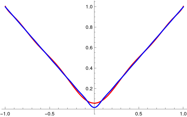
Figure 6.1: Chebyshev approximations with n = 5 terms (red) and n = 20 terms (blue).
As you can observe, even five term approximation gives a reasonable accuracy.
Theorem 4 (in this Chebyshev setting) says that the corresponding series converges in the mean.
Therefore:
The Chebyshev–Fourier series of |x| is infinite.
The partial sums SN are Chebyshev polynomials (finite combinations of Tₙ).
These polynomials approximate |x| in the mean square sense with respect to the weight w(x) = 1/√(1-x²).
The 𝔏2w-error of approximation goes to zero as N → ∞.
That is exactly Theorem 4 in a concrete, nontrivial, infinite‑series example.
■
End of Example 6
Theorem 5: (Uniqueness of Fourier Coefficients)
Let ℌ be a Hilbert space and let { ωₙ(x) } be a complete orthonormal system in ℌ. If f ∈ ℌ, then the Fourier coefficients
\[
a_n = \langle f, \omega_n \rangle
\]
uniquely determine f (up to equality almost everywhere in the 𝔏² case).
Equivalently:
If f,g ∈ ℌ satisfy
\[
\langle f, \omega_n \rangle = \langle g, \omega_n \rangle \qquad \forall n ,
\]
then
\[
f = g \quad \mbox{in } ℌ ,
\]
In 𝔏²-spaces, this means
\[
f(x) = g(x) \quad \mbox{ almost everywhere}.
\]
Suppose that two functions, f and g, have the same expansion coefficients, that is,
\[
a_k = \langle \omega_k , f \rangle = \langle \omega_k , g \rangle .
\]
Hence, ⟨ ωk , f − g ⟩ = 0, so by Theorem 3, f − g = 0, giving f = g
Now consider the converse problem. Does a given function have unique set of expansion coefficients? Assume that
\[
\lim_{n\to\infty} \left\| f - \sum_{k=1}^n a_k \omega_k \right\| = \lim_{n\to\infty} \left\| f - \sum_{k=1}^n b_k \omega_k \right\| ;
\]
that is, assume that there are two partial sums with different expansion coefficients that converge in the mean to the same function f. If the expansion coefficients are unique, then 𝑎ₙ = bₙ for all n. To prove this, we observe that
\begin{align*}
\left\| \sum_{k=1}^n a_k \omega_k -\sum_{k=1}^n b_k \omega_k \right\| &= \left\| \sum_{k=1}^n a_k \omega_k - f + f - \sum_{k=1}^n b_k \omega_k \right\|
\\
&\le \left\| f - \sum_{k=1}^n a_k \omega_k \right\| + \left\| f - \sum_{k=1}^n b_k \omega_k \right\| ,
\end{align*}
where we have used the triangle inequality. Now given any ε, we can choose by assumption an n large enough so that both the last two norms are less than ε/2. Therefore, for such an n,
\[
\left\| \sum_{k=1}^n a_k \omega_k - \sum_{k=1}^n b_k \omega_k \right\| = \left\| \sum_{k=1}^n \left( a_k - b_k \right) \omega_k \right\| = \left[ \sum_{k=1}^n \left( a_k - b_k \right)^2 \right]^{1/2} < \varepsilon .
\]
However, this can only be true if 𝑎ₙ = bₙ. So the expansion coefficients of a given function are unique. Since the set { ωₙ(x) } is complete orthonormal system of functions, it follows that 𝑎ₙ = bₙ = ⟨ ωₙ , f ⟩, the Fourier coefficients.
Example 7:
Chebyshev polynomials of the second kind satisfy
\[
U_n(\cos \theta )=\frac{\sin ((n+1)\theta )}{\sin \theta } = \sum_{i=0}^n P_{n-i} \left( \cos\theta\right) P_i \left( \cos\theta\right) ,
\]
Simplify[
Sum[LegendreP[4 - i, Cos[t]]*LegendreP[i, Cos[t]], {i, 0, 4}]]
1 + 2 Cos[2 t] + 2 Cos[4 t]
Simplify[ChebyshevU[4, Cos[t]]]
1 + 2 Cos[2 t] + 2 Cos[4 t]
where Pi is the Legendre polynomial of degree i.
The Chebyshev polynomials of second kind are orthogonal on [-1,1] with weight
\[
w(x)=\sqrt{1-x^2}.
\]
Define the Hilbert space
ℌ = 𝔏²([-1,1], w(x) dx), with inner product
\[
\langle f,g\rangle =\int _{-1}^1f(x)g(x)\sqrt{1-x^2}\, {\text d}x.
\]
The orthogonality relation becomes
\[
\int _{-1}^1U_m(x)U_n(x)\sqrt{1-x^2}\, {\text d}x = \frac{\pi }{2}\, \delta _{mn} ,
\]
where δmn is the Kronecker delta.
Thus, an orthonormal system is
\[
\omega _n(x)=\sqrt{\frac{2}{\pi }}\, U_n(x),\qquad n\geq 0.
\]
This system is complete in ℌ, so Theorem 4 applies.
Let’s take f(x) = |x|.
This function is even, continuous, and non‑polynomial — perfect for an infinite Chebyshev‑Uₙ expansion.
So Mathematica tells us that
\[
a_n = \sqrt{\frac{2}{\pi }}\, \frac{-2}{-3 + 2 n + n^2}\,\cos \left( \frac{n\pi}{2} \right) = \sqrt{\frac{2}{\pi }}\, \frac{-2}{(n-1)(n+3)} \times \begin{cases} 0, & \quad \mbox{if $n$ is odd},
\\
(-1)^k & \quad \mbox{if }\ n= 2k, \quad k=0,1,2,\ldots .
\end{cases}
\]
Because |cosθ| is even around π/2, only even n survive.
A classical Fourier computation yields the explicit formula:
\[
a_{2k+1} = 0,\qquad a_{2k} = -2\sqrt{\frac{2}{\pi}}\cdot \frac{(-1)^k}{(2k-1)(2k+3)}.
\]
Thus, the Fourier–Chebyshev series is genuinely infinite.
Putting the coefficients together, we obtain
\[
|x|\sim \sum _{k=0}^{\infty }a_{2k}\, \omega _{2k}(x) = -\frac{4}{\pi}\, \sum _{k=0}^{\infty} \frac{(-1)^k}{(2k-1)(2k+3)} \, U_{2k}(x).
\]
This is a true infinite series — it does not terminate.
For illustration of Theorem 4, we define the partial sums
\[
S_N(x) =\sum _{n=0}^N a_n\, \omega _n(x).
\]
We use Mathematica to plot some partial sums with 5 and 20 terms.
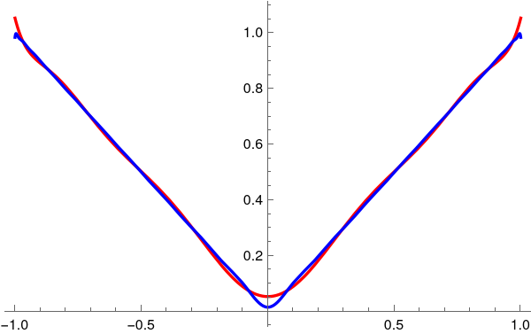
Figure 7.1: Chebyshev-2 approximations with n = 5 terms (red) and n = 20 terms (blue).
Each partial sum SN is a (finite) linear combination of Chebyshev polynomial of the second kind.
These polynomials approximate |x| in the mean‑square sense with respect to the weight √(1-x²).
The approximation improves monotonically as N → ∞.
The infinite series converges in the exact sense guaranteed by Theorem 4.
We present another illustrative example of Theorem 4 using Chebyshev polynomials of the third kind, usually denoted by Vₙ(x).
This gives you a genuinely infinite Fourier–Chebyshev expansion in a weighted Hilbert space, exactly parallel to the Uₙ example.
Chebyshev polynomials of the third kind Vₙ form an orthogonal system in the
Hilbert space ℌ = 𝔏⊃([−1, 1], w dx) with weight
\[
w(x) = (1 - x)^{-1/2} \cdot (1 + x)^{1/2} = \sqrt{\frac{1+x}{1-x}} .
\]
Chebyshev polynomials of the third kind Vₙ(x) are defined by either the recurrence relation
\[
\begin{split}
V_{n+1}(x) &= 2x \, V_n(x) - V_{n-1}(x) , \qquad n = 1,2,\ldots ,
\\
V_0 (x) &= 1 , \quad
V_1 (x) = 2x - 1,
\end{split}
\]
or via Chebyshev polynomials of the first and second kind
\[
V_n (x) = T_n (x) - \left( 1-x \right) U_{n-1}(x) ,
\]
or through Jacobi polynomials
\[
V_n (x) = \frac{n!}{(1/2)_n}\, P_n^{(-1/2, 1/2)}(x) = \frac{P_n^{(-1/2, 1/2)}(x)}{P_n^{(-1/2, 1/2)}(1)} = \frac{4^n \left( n! \right)^2}{(2n)!}\,P_n^{(-1/2, 1/2)}(x) ,
\]
where (1/2)ₙ is the Pochhammer symbol (rising factorial).
Similar to other Chebyshev polynomials, we can express Vₙ as
\[
V_{n} (\cos\theta ) = \frac{\cos \left( \frac{2n+1}{2}\,\theta \right)}{\cos \left( \frac{\theta}{2} \right)} .
\]
Chebyshev polynomials of the third kind are orthogonal on [-1,1] with weight
\[
w(x) = (1 - x)^{-1/2} \cdot (1 + x)^{1/2} = \sqrt{\frac{1+x}{1-x}} .
\]
Then the inner product in ℌ is
\[
\langle f,g\rangle =\int_{-1}^1 f(x)\,g(x)\, w(x)\, {\text d}x = \int_{-1}^1 f(x)\,g(x)\, \sqrt{\frac{1+x}{1-x}} \, {\text d}x .
\]
The orthogonality relation becomes
\[
\int _{-1}^1 V_m(x)\,V_n(x)\, w(x)\, {\text d}x =\frac{\pi }{2}\, \delta _{mn}.
\]
Thus, the corresponding orthonormal system becomes
\[
\omega _n(x) =\sqrt{\frac{2}{\pi}}\, V_n(x),\qquad n\geq 0.
\]
This system is complete in ℌ = 𝔏²([−1,1], wdx), so Theorem 4 applies. The Fourier coefficients are determined as
\[
a_n = \langle f, \omega_n \rangle = \sqrt{\frac{2}{\pi}} \int_0^{\pi} f(\cos\theta )\,2\cos\left( \frac{\theta}{2} \right) \cos \left( n + \frac{1}{2} \right) \theta \,{\text d}\theta , \quad n=0,1,2,\ldots .
\]
For function f(x) = |x|, Mathematica evaliate
\[
a_n = \sqrt{\frac{2}{\pi}} \cdot \frac{1}{n \left( n^2 -1 \right) \left( n+2 \right)} \left[ 2n^2 \sin \left( \frac{n\pi}{2} \right) -4n\,\cos \left( \frac{n\pi}{2} \right) -2n^2 \cos \left( \frac{n\pi}{2} \right) -2\,\sin\left( \frac{n\pi}{2} \right) \right] , \quad n\ge 2 .
\]
which we simplify using trigonometric identities, This gives
\[
a_n = \sqrt{\frac{2}{\pi }}\int_{0}^{\pi} \sqrt{2}\left( 1 + \cos\theta \right)\cos (n + 1/2)\theta )\,{\text d}\theta .
\]
Now we ask Mathematica to evaluate the integral:
This is exactly the same output when Mathematica was applied to unsimplified expression
\[
\sqrt{1+x} \,\sim\, \frac{2}{\pi} \sum_{n\ge 0} \frac{8\sqrt{2} (-1)^n}{3 + 2 n - 12 n^2 - 8 n^3} \,V_n (x) .
\]
Define partial sums
\[
S_N(x)=\sum _{n=0}^N a_n\, \omega _n(x) = \sqrt{\frac{2}{\pi}} \sum _{n=0}^N a_n\,V_n (x) ,
\]
Interpretation:
Each S_N is a finite Chebyshev polynomial of the third kind.
These polynomials approximate \sqrt{1+x} in the mean‑square sense with respect to the weight w(x)=1/(\sqrt{1-x^2}(1+x)).
The approximation improves monotonically as N → ∞.
The infinite series converges exactly as Theorem 4 guarantees.
This is a perfect demonstration of Theorem 4 using the third‑kind Chebyshev system, with a non‑polynomial function and a true infinite Fourier expansion.
■
End of Example 7
A subset \( \displaystyle \ \mathcal{D} \ \) of a Hilbert space ℌ is dense if every element of ℌ can be approximated arbitrarily well (in the norm of ℌ) by elements of \( \displaystyle \ \mathcal{D}. \ \) Concretely, for every f ∈ ℌ and every ε > 0, there exists g ∈ \( \displaystyle \mathcal{D} \quad \) with
\[
\| f-g\|_H < \varepsilon .
\]
This is the analytic expression of the geometric idea that \( \displaystyle \quad \mathcal{D} \quad \) “fills” the space: no nonzero vector is orthogonal to all of \( \displaystyle \quad \mathcal{D}. \quad \) Equivalently,
\[
\overline{\mathcal{D}} = ℌ\quad \Longleftrightarrow \quad \mathcal{D}^{\perp } = \{ 0\} .
\]
Completeness of an orthogonal system { ϕₙ } ⊆ ℌ means that its finite linear combinations form a dense set. In that case, every f ∈ ℌ admits a convergent Fourier expansion
\[
f\sim \sum _{n=0}^{\infty }c_n\phi _n,
\]
with convergence in the norm of ℌ. This is the setting in which Parseval’s identity and the usual Fourier approximation theory operate.
provides a typical example of a complete orthogonal system in Hilbert space 𝔏²([−π, π]) of square integrable functions on any interval of length 2π. Functions in this system are not normalized, so we need to divide each of them by corresponding norm to obtain the orthonormal set of functions:
The trigonometric system is therefore the canonical model of a complete orthogonal system. Its density also follows from the Sturm--Liouville theory. Indeed, let us consider the unbounded differential operator
\[
L=-\frac{{\text d}^2}{{\text d}x^2}
\]
on Hilbert space ℌ = 𝔏²(−π, π) with periodic boundary conditions
This is a self‑adjoint positive operator on a Hilbert space ℌ. Its eigenfunctions are exactly \eqref{EqOrtho.1} with eigenvalues {n²}. The spectral theory says that for such a regular self‑adjoint problem on a finite interval, the eigenfunctions form a complete orthogonal set in 𝔏². “Complete” here means their closed linear span is the whole space. So the trigonometric system is dense in 𝔏²(−π,π) because it is the eigenbasis of a self‑adjoint operator with discrete spectrum.
Theorem 6:
An orthonormal system { ωₙ(x) } in Hilbert space ℌ is closed if and only if Parseval's identity holds for a dense family of functions.
Necessary condition is obvious.
We need to prove only its sufficience. Let us consider operation Sₙ that transfers a function f(x) into a linear combination spanned on first n functions ω₁ , ω₂ , … , ωₙ by calculating n-th partial Fourier sum Sₙ(f; x). This transformation satisfies the following properties:
Sₙ(f₁ + f₂) = Sₙ(f₁) + Sₙ(f₂);
Sₙ(λ f) = λ Sₙ(f), λ ∈ ℂ;
∥Sₙ(f)∥ ≤ ∥f∥.
Property "a" reflects the fact that the Fourier coefficient of a sum of two functions is the sum of Fourier coefficients of corresponding functions, which follows from the corresponding property of inner product. This is also true for property "b". Property "c" is just a finite version of Bessel's inequality:
\[
\sum_{i=1}^n \left\vert \langle f , \omega_i \rangle \right\vert^2 \le \| f \|^2 .
\]
For any ε > 0 and any function f ∈ 𝔏², find a function g(x) from a dense set A such that
\[
\| f - g \| < \frac{\varepsilon}{3} .
\]
Since for functions from family A the closeness condition is valid, there exists an integer N such that for n ≥ N, we have
\[
\| g - S_n (g) \| \le \frac{\varepsilon}{3} .
\]
Let us estimate the norm of the difference:
\begin{align*}
\| f - S_n (f) \| &= \| f -g + g - S_n (g) + S_n (g) - S_n (f) \|
\\
&\leqslant \| f - g \| + \| g - S_n (g) \| + \| S_n (g) - S_n (f) \|
\\
&\leqslant 2 \| f - g \| + \| g - S_n (g) \| < \varepsilon
\end{align*}
for n ≥ N.
Before we work on the nest example, we need some preliminary information.
A function f : [0,1] → ℝ is a dyadic step function if there exists some integer N such that:
\[
f(x) = c_n\quad \mathrm{for\ }x\in \left[ \frac{n}{2^N},\, \frac{n+1}{2^N}\right) ,\qquad n=0,1,\dots ,2^N -1.
\]
The constants cₙ can be arbitrary real numbers.
The following dyadic function
\[
\psi (x) = \begin{cases}
1, &\quad \mbox{for } 0 \le x < 1/2 , \\
-1 &\quad \mbox{for } 1/2 \le x < 1 , \\
0, &\quad \mbox{elsewhere.}
\end{cases}
\]
is called the mother wavelet or the Haar function..
A dyadic step function is a step function whose “steps’’ occur at dyadic rationals, meaning numbers of the form
\[
\frac{k}{2^n},\qquad k,n\in \mathbb{Z}.
\]
It is one of the fundamental building blocks in analysis, probability, and harmonic analysis because it aligns perfectly with binary subdivision of the interval. A dyadic step function on an interval (usually [0,1]) is a function that is:
Piecewise constant.
Constant on each dyadic interval
\[
I_{n,k}=\left[ \frac{k}{2^n},\, \frac{k+1}{2^n}\right) .
\]
Allowed to jump only at dyadic points \( \displaystyle \quad \frac{k}{2^n}. \)
Example 8:
Let ℌ = 𝔏²(ℝ), with usuall inner product.
Define the Haar mother wavelet:
\[
\psi _{j,k}(x)=2^{j/2}\, \psi (2^jx-k)
\]
for j,k ∈ ℤ.
Then { ψj,k }j,k ∈ ℤ is an orthonormal system in 𝔏²(ℝ).
It is a dense family in ℌ where Parseval's identity holds.
Let us consider the set
\[
\mathcal{D} = \left\{ f\in 𝔏^2(\mathbb{R}):f\mathrm{\ has\ compact\ support\ and\ is\ piecewise\ constant\ on\ dyadic\ intervals\ }[m2^{-N},(m+1)2^{-N})\right\} .
\]
These dyadic step functions are dense in 𝔏²(ℝ) (they approximate any 𝔏² function by local averaging on fine dyadic grids).
Wavelet expansion on \( \displaystyle \quad \mathcal{D}\ : \ \) For such an f, only finitely many Haar coefficients
\[
c_{j,k}=\langle f,\psi _{j,k}\rangle
\]
are nonzero, because f is constant on sufficiently fine dyadic intervals and has compact support.
Parseval's identity on \( \displaystyle \quad \mathcal{D}: \ \) For each \( \displaystyle \quad f\in \mathcal{D}, \)
\[
\| f\| _{𝔏^2(\mathbb{R})}^2=\sum _{j,k}|\langle f,\psi _{j,k}\rangle |^2,
\]
where the sum is actually finite (so there is no convergence issue).
Thus Parseval’s identity holds for all f in the dense set \( \displaystyle \quad \mathcal{D}. \)
Theorem 6 says:
An orthonormal system { ωₙ } in ℌ is closed (complete) if and only if Parseval’s identity holds for a dense family of functions.
We have: { ψj,k } is orthonormal in 𝔏²(ℝ).
There is a dense set \( \displaystyle \quad \mathcal{D} \subset 𝔏^2(\mathbb{R}) \) (dyadic step functions) such that Parseval's identity holds for every \( \displaystyle \quad f\in \mathcal{D}. \)
Therefore, by Theorem 6, the Haar wavelet system { ψj,k } is closed, i.e., complete in 𝔏²(ℝ).
We have:
{ ψj,k } is orthonormal in 𝔏²(ℝ).
There is a dense set \( \displaystyle \quad \mathcal{D} \subset 𝔏^2;(\mathbb{R}) \) (dyadic step functions) such that Parseval holds for every f ∈ \( \displaystyle \quad \mathcal{D}. \)
Therefore, by Theorem 6, the Haar wavelet system { ψj,k } is closed, i.e., complete in 𝔏²(ℝ).
■
For given finite list of functions { ϕ₁, ϕ₂, … , ϕₙ } and scalars b₁, b₂, … , bₙ, the xpression
\[
b_1 \phi_1 + b_2 \phi_2 + \cdots + b_n \phi_n
\]
is called the linear combination funxtions ϕ₁, ϕ₂, … , ϕₙ.
A set of funxtions ϕ₁, ϕ₂, … , ϕₙ is called linear independent if no function in the set can be expressed as a linear combination (constant multiple) of the others. A set of functions is linearly independent if b₁ϕ₁ + b₂ϕ₂ + ⋯ + bₙϕₙ = 0 mplies all constants bi
are zero.
An (infinite) set of functions { ϕₙ }, n = 1, 2, … , is called linearly independent if any finite subset of these functions is linearly independent.
Suppose we know a basis { ϕₙ }ₙ≥1 in a separable Hilbert space ℌ with inner product ⟨·∣·⟩. This means that elements in the system { ϕₙ } are linearly independent and the set of all finite linear combinations \( \displaystyle \ \sum_{i=1}^n c_i \phi_i , \ \) where coefficients ci are arbitrary scalars and integer n can be any number, form a dense subset in ℌ.
We are going to find an orthogonal basis { ψₙ } using Gram–Schmidt process. We start with a basis of two elements { ϕ₁, ϕ₂ } that are linearly independent. let us take the first of them as our first element in a new orthogonal basis, so let ψ₁ = ϕ₁. As our next vector, we choose a difference between ϕ₂ and its projection on ϕ₁:
This vector ψ₂ is linearly independent of ψ₁ because it is not a scalar multiple of ψ₁ = ϕ₁, but it is a linear combination of two elements, ϕ₁ and ϕ₂. This observation is a core of orthogonalization.
For arbitrary n ∈ ℤ, we build a system of n elements { ψψ₁, ψ₂, … , ψₙ } that is linearly independent and mutually orthogonal:
Our objective is to determine coefficients bi,j in such a way that vectors ψ₁, ψ₂, … , ψₙ are non-zero and mutually orthogonal (then they will be linearly independent). In other words, the list of n elements { ψ₁, ψ₂, … , ψₙ } forms an orthogonal basis for the span of
{ ϕ₁, ϕ₂, … , ϕₙ }. We build the required system { ψ₁, ψ₂, … , ψₙ } inductively. Suppose that such system of n elements has been already determined. We seek the next element ψn+1 as a linear combination:
because the list { ψ₁, ψ₂, … , ψₙ } is mutually orthogonal by construction. Since ⟨ ψi ∣ ψi ⟩ = ∥ψi∥² ≠ 0, the above equation has a unique solution, ci. Hence, vector ψn+1 is orthogonal to all previously determined elements { ψ₁, ψ₂, … , ψₙ }. Moreover, this vector ψn+1 is non-zero. Indeed, substituting into the formula
This expression cannot be zero because elements in the list { ϕ₁, ϕ₂, … , ϕₙ, ϕn+1 } are linearly independent, and the right hand-side is just their linear combination.
Now we prove that the system { ϕ₁, ϕ₂, … , ϕₙ, …} is complete. Choose arbitrary f ∈ ℌ and ε > 0. Since the set of all linear combinations
\( \displaystyle \ \sum_{k=1}^n c_k \phi_k \ \) is dense in ℌ, then there exist scalars b₁, b₂, … , bₙ and integer n such that
\[
\left\| f - \sum_{k=1}^n a_k \omega_k \right\| \le \left\| f - \sum_{k=1}^n d_k \omega_k \right\| < \varepsilon ,
\]
where 𝑎i = ⟨ f∣ωi ⟩ are Fourier coefficients of function f. This means that the orthogonal systems { ωi } and so { ψi } are complete.
Let 𝒫⟦x⟧ be a set of all polynomials with real coefficients and 𝒫≤n⟦x⟧ be its subset of polynomials of degree up to n. Both these vector spaces have a basis (in the usual sense), consisting of monomials 1, x, x², x³, …, which terminates for 𝒫≤n⟦x⟧.
However, the Stone---Weierstrass theorem would be false if it claimed to produce a uniformly convergent power series, known as Taylor's serries. For instance, these is no power series that converges uniformly to the continuous function √x in the interval [0,1]. Taylor series are beautiful theoretically and essential in analysis, but numerically they are too fragile, especially for practical numerical approximations because they behave poorly outside a narrow region and are expensive or unstable to compute. The core issue is that Taylor series are local objects, while numerical approximations usually need global stability and accuracy.
Weierstrass's theorem for approximations by a sequence of polynomials is in one sense much stronger than Taylor's theorem for expansion in power series. Weierstrass's theorem demonstrates the existence of polynomial approximations outside the radius of convergence of a Taylor series. However, there is, in general, no possibility of rearranging the uniform convergent sequence of polynomials that approximate any continuous function as to produce a convergent Taylor's series. Therefore, polynomials are more suitable for approximations than power series. The follwoing examples demonstrate how we can generate orthogonal polynomials from the set of monomials { xⁿ }n≥0 using the Gram–Schmidt process.
Gram-Schmidt orthogonalization is a method that takes a non-orthogonal set of
linearly independent function and literally constructs an orthogonal set over an arbitrary
interval and with respect to an arbitrary weighting function. Here for convenience, all
functions are assumed to be real.
Example 9:
The Legendre polynomials appear in many different contenxts, so they can be defined, for instance, via the Rodrigues' formula
\[
P_n (x) = \frac{1}{2^n n!}\,\frac{{\text d}^n}{{\text d}x^n} \left( x^2 -1 \right)^n = \frac{1}{2^n}\,\sum_0^{\lfloor n/2 \rfloor} (-1)^{k} \frac{(2n-2k)!}{k! \,(n-k)! \, (n-2k)!}\, x^{n-2k} ,
\]
or by recurrence
\[
\left( n+1 \right) P_{n+1} (x) = \left( 2n+1 \right) P_n - n\,P_{n-1} (x) , \qquad P_0 = 1, \quad P_1 (x) = x .
\]
The polynomials were named "Legendre coefficients" by the British mathematician Isaac Todhunter in honor of the French mathematician Adrien-Marie Legendre (1752–1833), who was the first to introduce and study them. Todhunter called the functions "coefficients", instead of "polynomials", because they appear as coefficients in the expansion of the generating function; Todhunter also introduced the notation Pₙ, which is still generally used.
Legendre's polynomials have been introduced by Legendre in a memoir Sur l'attraction des sphéroïdes homogènes published in the Mémoires de Mathématiques et de Physique, présentés à l'Académie royale des sciences par sçavants étrangers, Tome x, pp. 411–435, Paris, 1785.
■
End of Example 9
Example 10:
■
End of Example 10
Example 11:
Like the other classical orthogonal polynomials, the Hermite polynomials can be defined from several different starting points. In this example, we use orthogonalization procedure to derive these polynomials. They were invented and studied in detail by the Russian scientist Pafnuty Chebyshev in 1859. Five years later, Charles Hermite provided a deep analysis of these polynomials. Therefore, they were known for almost 100 years as Chebyshev--Hermite polynomials.
It should be noted that these polynomials were mentioned previously in 1810 by Pierre-Simon Laplace in scarcely recognizable form.
Hermite polynomials, denoted by Hₙ(x), can be defined recursively
\[
H_{n+1} (x) = 2x\,H_n (x) - 2n\,H_{n-1} (x) , \qquad H_0 (x) = 1, \quad H_1 (x) = 2x.
\]
Mathematica has a build-in command:
Figure 11.1: Hermite polynomial H₅(x) on real axis.
Figure 11.2: Hermite polynomial H₅(z) for complex variable.
Be aware that there are the "probabilist's Hermite polynomials", given by
\[
\mbox{He}_n ( x ) = ( − 1 )^n e^{x^2 /2} \frac{{\text d}^n}{{\text d} x^n}\, e^{− x^2 /2} , \qquad n=0,1,2,\ldots .
\]
The Hermite polynomial Hₙ(x) can be derived by orthogonalization of the list of monomials
\[
\phi_n (x) = x^n \qquad \left( n=0,1,2,\ldots \right) ,
\]
with the weight function
\[
w(x) = e^{-x^2} .
\]
These monomials { xⁿ } are linearly independent, but not orthogonal. We verify their linearly independence with Mathematica by showing that their Wronskian is not zero.
Starting with n = 0, let
\[
\psi_0 = \phi_0 = 1 , \quad \omega_0 = \frac{1}{\| 1 \|} = \frac{1}{\pi^{1/4}}
\]
because
\[
\int_{-\infty}^{\infty} {\text d} x =
\]
Integrate[Exp[-x^2], {x, -Infinity, Infinity}]
Sqrt[\[Pi]]
For n = 1, let
\[
\psi_1 = \phi_1 + b_{10}\phi_0 = x + b_{10} .
\]
This function is orthogonal to ϕ₀ if its inner product with this function vanishes:
\[
0 = \langla \psi_1 \mid \phi_0 \rangle = \int_{-\infty}^{\infty} \left( x + b_{10} \right) e^{-x^2} {\text d} x = b_{10} \int_{-\infty}^{\infty} e^{-x^2} {\text d} x .
\]
Since the integral of b10 is non-zero, we conclude that b10 = 0. Hence, ψ₁ = x.
For n = 2, let
\[
\psi_2 = \phi_2 + b_{20}\phi_0 + b_{21} \phi_1 = x^2 + b_{20} + b_{21} x .
\]
Its inner product with ϕ₀ = 1 gives
\[
0 = \langle \psi_2 \mid 1 \rangle = \int_{-\infty}^{\infty} \left( x^2 + b_{20} + b_{21} x \right) {\text d} x = b_{20} \sqrt{\pi} + \frac{\sqrt{\pi}}{2} .
\]
For n = 2, let
\[
\psi_3 = \phi_3 + b_{30}\phi_0 + b_{31} \phi_1 +b_{32} \phi_2 = x^3 + b_{32} x^2 + b_{31} x + b_{30} .
\]
Taking the inner prosuct with 1, we get
\[
0 = \langle \psi_3 \mid 1 \rangle = b_{30} \| 1 \|^2 + b_{32} \langle x^2 \mid 1 \rangle .
\]
Similarly, we have
\begin{align*}
0 &= \langle \psi_3 \mid x \rangle = b_{31} \langle x \mid x \rangle + \langle x^3 \mid x \rangle ,
\\
0 &= \langle \psi_3 \mid x^2 \rangle = b_{32} \langle x^2 \mid x^2 \rangle + b_{30} \langle 1 \mid x^2 \rangle ,
\\
0 &= \langle \psi_3 \mid x^3 \rangle = b_{32} \langle x^2 \mid x^2 \rangle +
\end{align*}
■
End of Example 11
Byron, F.W. and Fuller, R.W., Mathematics of Classical and Quantum Physics, Dover Publications, 1992.
I. Todhunter, An Elementary Treatise on Laplace's, Lamé's, and Bessel's Functions, MacMillan, 1875 (London).
Return to Mathematica page
Return to the main page (APMA0340)
Return to the Part 1 Basic Concepts
Return to the Part 2 Fourier Series
Return to the Part 3 Integral Transformations
Return to the Part 4 Parabolic PDEs
Return to the Part 5 Hyperbolic PDEs
Return to the Part 6 Elliptic PDEs
Return to the Part 6P Potential Theory
Return to the Part 7 Numerical Methods