To enhance pedagogical effectiveness, the treatment of the dot product is presented in several distinct sections

Solvability

Let us consider a system of linear equations written in succinct matrix-vector form:

\begin{equation} \label{EqDot.1} \mathbf{A}\,\mathbf{x} = \mathbf{b} , \qquad \mathbf{A} \in \mathbb{F}^{m\times n}, \quad \mathbf{x} \in \mathbb{F}^{n\times 1}, \quad \mathbf{b} \in \mathbb{F}^{m\times 1}, \end{equation}

where A is an m-by-n matrix with entries from a field 𝔽 (the set of real or complex numbers), x is an n × 1 column vector representing n unknowns, and b is a given m × 1 column vector. In fact, any linear transformation between finite-dimensional vector spaces X and Y (where dim(X) = n and dim(Y) = m) over the field 𝔽 can be expressed in the matrix-vector form \eqref{EqDot.1} upon choosing coordinates with respect to fixed bases in X and Y.

We remind some notations.

Every m-by-n matrix A ∈ 𝔽^m×n defines, a linear transformation T_A : 𝔽^{n × 1} ⇾ 𝔽^{m × 1} by multiplication from left: T_A(x) = A x. Then:

kernel (also known as the null space): ker(A) = {x ∈ 𝔽^{n × 1} : A x = 0} ⊆ 𝔽^{n × 1};
image: im(A) = {A x : x ∈ 𝔽^{n × 1}} ⊆ 𝔽^{m × 1}; it is known in the matrix theory as the column space, denoted by 𝒞(A);
cokernel is the factor space: coker(A) = 𝔽^{m × 1}/image(A);
left-null space: ker(Aᵀ), which is the kernel of the transpose matrix;
coimage: is the quotient space: coim(A) = 𝔽ⁿ/ker(A).

Suppose that the matrix A is composed of n column vectors:

\[ \mathbf{A} = \begin{bmatrix} \mathbf{a}_1 & \mathbf{a}_2 & \cdots & \mathbf{a}_n \end{bmatrix} , \]

where each aₖ ∈ 𝔽^{m × 1} is the k-th column of the matrix A for k = 1, 2, … ,n. Then, the matrix-vector product A x can be expressed as a linear combination of the columns of A:

\[ \mathbf{A}\mathbf{x} = x_1 \mathbf{a}_1 + x_2 \mathbf{a}_2 + \cdots + x_n \mathbf{a}_n = \mathbf{b} \in \mathbb{F}^{m\times 1} . \]

The equation above means that b is a vector in span{a₁, a₂, … , a_n}. This formulation highlights that solving the equation A x = b is equivalent to finding scalars (x₁, x₂, … , xₙ) such that the linear combination of the column vectors of A equals the target vector b. Consequently, a solution exists if and only if b is an element of the subspace generated by the column vectors of the matrix A. This subspace is referred to as the column space, denoted by 𝒞(A), or the image of A.

Example 51: To enhance understanding of the left null space, we consider a 2-by-3 matrix that we fill with some integers: \[ \mathbf{A} = \begin{bmatrix} a_{1,1} & a_{1,2} & a_{1,3} \\ a_{2,1} & a_{2,2} & a_{2,3} \end{bmatrix} , \qquad \mathbf{A} = \begin{bmatrix} 1&2&3 \\ 4&5&6 \end{bmatrix} . \tag{2.1} \] Its transpose is \[ \mathbf{A}^{\mathrm T} = \begin{bmatrix} a_{1,1} & a_{2,1} \\ a_{1,2} & a_{2,2} \\ a_{1,3} & a_{2.3} \end{bmatrix} , \qquad \mathbf{A}^{\mathrm T} = \begin{bmatrix} 1&4 \\ 2&5 \\ 3&6 \end{bmatrix} \tag{2.2} \] Matrix A ∈ 𝔽^m×n can be represented as a row of column vectors: \[ \mathbf{A} = \begin{bmatrix} {\bf a}_1 & {\bf a}_2 & \cdots & {\bf a}_n \end{bmatrix} , \] where in our case of m = 2 and n = 3, we have \[ \mathbf{a}_1 = \begin{pmatrix} a_{1,1} \\ a_{2,1} \end{pmatrix} = \begin{pmatrix} 1 \\ 4 \end{pmatrix} , \quad \mathbf{a}_2 = \begin{pmatrix} a_{1,2} \\ a_{2,2} \end{pmatrix} = \begin{pmatrix} 2 \\ 5 \end{pmatrix} , \quad \] and \[ \mathbf{a}_3 = \begin{pmatrix} a_{1,3} \\ a_{2,3} \end{pmatrix} = \begin{pmatrix} 3 \\ 6 \end{pmatrix} \] We can find a similar representation for the transpose matrix \[ \mathbf{A}^{\mathrm T} = \begin{bmatrix} {\bf a}_1^{\mathrm T} & {\bf a}_2^{\mathrm T} & \cdots & {\bf a}_m^{\mathrm T} \end{bmatrix} , \] where \[ {\bf a}_1^{\mathrm T} = \begin{pmatrix} a_{1,1} \\ a_{1,2} \\ a_{1,3} \end{pmatrix} = \begin{pmatrix} 1 \\ 2 \\ 3 \end{pmatrix} , \quad {\bf a}_2^{\mathrm T} = \begin{pmatrix} a_{2,1} \\ a_{2,2} \\ a_{2,3} \end{pmatrix} = \begin{pmatrix} 4 \\ 5 \\ 6 \end{pmatrix} . \] Then product of transpose matrix A^T and column vector z ∈ ℝ^2×1 can be written as \[ {\bf A}^{\mathrm T} \mathbf{z} = \begin{bmatrix} a_{1,1} & a_{2,1} \\ a_{1,2} & a_{2,2} \\ a_{1,3} & a_{2.3} \end{bmatrix} \begin{pmatrix} z_1 \\ z_2 \end{pmatrix} = \begin{pmatrix} a_{1,1} z_1 + a_{2,1} z_2 \\ a_{1,2} z_1 + a_{2,2} z_2 \\ a_{1,3} z_1 + a_{2,3} z_2 \end{pmatrix} . \] Using column vectors of matrix A^T, we rewrite it as \[ {\bf A}^{\mathrm T} \mathbf{z} = z_1 \begin{pmatrix} a_{1,1} \\ a_{1,2} \\ a_{1,3} \end{pmatrix} + z_2 \begin{pmatrix} a_{2,1} \\ a_{2,2} \\ a_{2,3} \end{pmatrix} = z_1 {\bf a}_1^{\mathrm T} + z_2 {\bf a}_2^{\mathrm T} . \] Hence, the left null space as a column space is \[ \mbox{ker}\left( \mathbf{A}^{\mathrm T} \right) = \left\{ \mathbf{z} \in \mathbb{F}^{m\times 1} \ : \quad \sum_{k=1}^m z_k \mathbf{a}_k^{\mathrm T} = 0 \right\} . \] For our 2-by-3 matrix, it becomes \[ \mbox{ker}\left( \mathbf{A}^{\mathrm T} \right) = \left\{ \mathbf{z} = \begin{pmatrix} z_1 \\ z_2 \end{pmatrix} \ : \quad z_1 \begin{pmatrix} 1 \\ 2 \\ 3 \end{pmatrix} + z_2 \begin{pmatrix} 4 \\ 5 \\ 6 \end{pmatrix} = 0 \right\} , \] which is equivalent to solving the following system of equations: \begin{align*} z_1 + 4 z_2 &= 0 , \\ 2 z_1 + 5 z_2 &=0 , \\ 3 z_1 + 6 z_2 &= 0 . \end{align*} From the first equation, we get z ₁n = −4z ₂. Substituting this expression into the remainder equations leads to to two equations \[ -8 z_2 + 5 z_2 = 0, \quad -4 z_2 + 2 z_2 = 0 \] These two equations have the only zero solution. Mathematica confirms:

AA = {{1, 2, 3}, {4, 5, 6}} NullSpace[Transpose[AA]]

{}

Now we represent the left null space as a row vector space. To achive this, we multiply matrix A by row vector y = [y₁, y₂] from left. This yields \[ \mathbf{y}\,\mathbf{A} = \begin{bmatrix} y_1 & y_2 \end{bmatrix} \begin{pmatrix} a_{1,1} & a_{1,2} & a_{1,3} \\ a_{2,1} & a_{2,2} & a_{2,3} \end{pmatrix} = \begin{bmatrix} y_1 a_{1,1} + y_2 a_{1,2} \\ y_1 a_{2,1} + y_2 a_{2,2} \\ y_1 a_{1,3} + y_2 a_{2,3} \end{bmatrix} \] Or \[ \mathbf{y}\,\mathbf{A} = y_1 \begin{bmatrix} a_{1,1} \\ a_{1,2} \\ a_{1,3} \end{bmatrix} + y_2 \begin{bmatrix} a_{1,2} \\ a_{2,2} \\ a_{2,3} \end{bmatrix} = y_1 \mathbf{a}_1^{\mathrm T} + y_2 \mathbf{a}_1^{\mathrm T} . \] Therefore, we can define the left null space as the row vector space: \[ \mbox{ker}\left( \mathbf{A}^{\mathrm T} \right) = \left\{ \mathbf{y} = \begin{bmatrix} y_1 & y_2 \end{bmatrix} \ : \quad y_1 \begin{pmatrix} 1 \\ 2 \\ 3 \end{pmatrix} + y_2 \begin{pmatrix} 4 \\ 5 \\ 6 \end{pmatrix} = 0 \right\} , \] which is exactly the same as column space.

■

End of Example 51

An Operational Interpretation via the Dot Product

In applied mathematics, computer science, and engineering, the dot product operator (•) is often abstracted beyond its basic definition between two single coordinate vectors. A prime example from vector calculus is the Laplacian operator, written symbolically as the operational dot product Δ = ∇ • ∇, where the nabla operator (∇) acts upon another copy of itself.

In a similar light, we can re-evaluate the matrix-vector product A x by partitioning A into its m row vectors rather than its columns:

\[ \mathbf{A} = \begin{bmatrix} \mathbf{r}_1^T \\ \mathbf{r}_2^T \\ \vdots \\ \mathbf{r}_m^T \end{bmatrix} \]

where each $ \displaystyle \quad \mathbf{r}_i^{\mathrm T} \quad $ represents a horizontal row vector in 𝔽^{1 × n}. When evaluating the equation A x = b, the matrix multiplication acts as a parallelized sequence of standard dot products between each row of the matrix and the column vector x:

\[ \mathbf{A}\mathbf{x} = \begin{bmatrix} \mathbf{r}_1 \cdot \mathbf{x} \\ \mathbf{r}_2 \cdot \mathbf{x} \\ \vdots \\ \mathbf{r}_m \cdot \mathbf{x} \end{bmatrix} = \begin{bmatrix} b_1 \\ b_2 \\ \vdots \\ b_m \end{bmatrix} = \mathbf{b} \]

In this framework, the matrix A behaves as an operator, and the matrix-vector product acts as a generalized dot product mapping an entry-wise collection of dual components. Understanding this operational perspective is vital for our upcoming work on duality and adjoint operators, where we will observe how these rows define hidden geometric constraints on the solvability of the entire system.

Definition (The Orthogonal Complement). Let S be a subset of ℝⁿ. The orthogonal complement of S, denoted by S^⊥ (pronounced “S-perp”), is the set of all vectors in ℝⁿ that are orthogonal to every vector in S with respect to the standard dot product:

\[ S^\perp = \{ \mathbf{x} \in \mathbb{R}^n : \mathbf{x} \cdot \mathbf{s} = 0 \text{ for every } \mathbf{s} \in S \} \]

More generally, if S is a subset of the complex vector space ℂⁿ, its orthogonal complement with respect to the standard complex inner product ⟨ ·∣· ⟩ is defined as:

\[ S^\perp = \{ \mathbf{x} \in \mathbb{C}^n : \langle \mathbf{x} \mid \mathbf{s} \rangle = 0 \text{ for every } \mathbf{s} \in S \} \]

The Necessary Condition for Solvability

The geometric structure of the orthogonal complement provides an immediate test for whether a system is solvable. Suppose we multiply both sides of our linear equation A x = b from the left by a row vector yᵀ ∈ 𝔽^{1 × m}, where y is chosen specifically from the left null space of A (meaning y ∈ ker(Aᵀ)). Using associative properties, this yields:

\[ \mathbf{y}^{\mathrm T} ( \mathbf{A}\mathbf{x} ) = ( \mathbf{A}^{\mathrm T} \mathbf{y} )^{\mathrm T} \mathbf{x} = \mathbf{y}^{\mathrm T} \mathbf{b} . \]

Since Aᵀy = 0 ∈ 𝔽^{n × 1}, the left side of the equation collapses entirely to zero, forcing an ultimate algebraic consistency constraint on the right side:

\[ \left[ 0 \right] = \mathbf{y}^{\mathrm T} \mathbf{b} \in \mathbb{F}^{1\times 1} \qquad \iff \qquad \mathbf{y} \cdot \mathbf{b} = 0 \]

This reveals a profound geometric absolute: if the system A x = b possesses a solution, then the target vector b must be orthogonal to every vector in the left null space of the matrix. If even a single vector y ∈ ker(Aᵀ) can be found such that y • b ≠ 0, a solution cannot physically exist.

Extension to Complex Fields and Inner Product Spaces

The exact test above based on dot products can be extended naturally to complex spaces ℂᵐ and ℂⁿ. Recall that j or ⅉ denotes the imaginary unit vector of the complex plane ℂ with ⅉ² = −1. When working over ℂ, the algebraic transpose is replaced by the conjugate transpose (or Hermitian adjoint), denoted as A^✶ (or Aᴴ). If we evaluate the compatibility test using the standard complex inner product, an identical mechanism emerges via the fundamental adjoint identity:

\[ \langle \mathbf{A}\mathbf{x}, \mathbf{y} \rangle = \langle \mathbf{x}, \mathbf{A}^*\mathbf{y} \rangle . \]

If we select a vector y from the complex left null space, ker(A^✶), such that A^✶y = 0, substituting it into the inner product yields:

\[ \langle \mathbf{b}, \mathbf{y} \rangle = \langle \mathbf{A}\mathbf{x}, \mathbf{y} \rangle = \langle \mathbf{x}, \mathbf{A}^*\mathbf{y} \rangle = \langle \mathbf{x}, \mathbf{0} \rangle = 0 . \]

Thus, regardless of whether the system is defined over real or complex fields, solvability is inherently bound to orthogonality. This relationship is codified cleanly by the direct-sum decompositions of our spaces:

\[ \mathbb{R}^n = \mathcal{C}(\mathbf{A}^{\mathrm T},) \oplus \ker(\mathbf{A}) \qquad \text{and} \qquad \mathbb{R}^m = \mathcal{C}(\mathbf{A}) \oplus \ker\left(\mathbf{A}^{\mathrm T}\right) , \] \[ \mathbb{C}^n = \mathcal{C}(\mathbf{A}^*) \oplus \ker(\mathbf{A}) \qquad \text{and} \qquad \mathbb{C}^m = \mathcal{C}(\mathbf{A}) \oplus \ker\left(\mathbf{A}^*\right) . \]

Here $ \displaystyle \quad \mathcal{C}(\mathbf{A}) \quad $ denotes the column space of matrix A, which we also denote as 𝒞(A).

Lemma 1 (Orthogonality of the Four Subspaces): Let A ∈ 𝔽^{m × n}.

If 𝔽 = ℝ, then every vector in the row space 𝒞(Aᵀ) is orthogonal to every vector in the null space, ker(A), with respect to the standard dot product. Similarly, every vector in the column space 𝒞(A) is orthogonal to every vector in the left null space, ker(Aᵀ).
If 𝔽 = ℂ, then every vector in the conjugate-row space 𝒞(A^✶) is orthogonal to every vector in the null space ker(A) with respect to the standard complex inner product. Similarly, every vector in the column space 𝒞(A) is orthogonal to every vector in the left null space ker(A^✶).

1. The Real Case (𝔽 = ℝ):

Row Space and Null Space (𝒞(Aᵀ) ⊥ ker(A)): Let x ∈ ker(A), meaning A x = 0. Let v be any vector in the row space 𝒞(Aᵀ). By definition, v can be expressed as a linear combination of the rows of A, which means v = Aᵀy for some vector y ∈ ℝᵐ (I am lazy to type "×1" in order to identify column vector). Taking the standard dot product of v and x:
\[ \langle \mathbf{v}, \mathbf{x} \rangle \Longrightarrow \mathbf{v}^{\mathrm T} \mathbf{x} = (\mathbf{A}^{\mathrm T} \mathbf{y})^{\mathrm T} \mathbf{x} = \mathbf{y}^{\mathrm T} (\mathbf{A}\mathbf{x}) . \]
Since x ∈ ker(A), we have A x = 0. Substituting this into equation above yields:
\[ \mathbf{y}^{\mathrm T} \mathbf{0} = 0 . \]
Thus, every vector in the row space is orthogonal to every vector in the null space.
Column Space and Left Null Space (𝒞(A) ⊥ ker(Aᵀ)): Let w ∈ ker(Aᵀ), meaning Aᵀ w = 0. Let b be any vector in the column space 𝒞(A), meaning b = A z for some vector z ∈ ℝⁿ. Taking their standard dot product:
\[ \langle \mathbf{w}, \mathbf{b} \rangle \g \Longrightarrow \mathbf{w}^{\mathrmT} \mathbf{b} = \mathbf{w}^{\mathrmT} (\mathbf{A}\mathbf{z}) = (\mathbf{A}^{\mathrmT} \mathbf{w})^{\mathrmT} \mathbf{z} . \]
Since Aᵀw = 0, this reduces directly to:
\[ \mathbf{0}^{\mathrm T} \mathbf{z} = 0 . \]
Thus, the left null space and the column space are completely orthogonal.

2. The Complex Case (𝔽 = ℂ):

The logic mirrors the real case exactly, substituting the standard complex inner product ⟨ u, v ⟩ = u^✶ v, where A^✶ represents the conjugate transpose (adjoint).

Conjugate-Row Space and Null Space (𝒞(A^✶) ⊥ ker(A)): Let x ∈ ker(A) (A x = 0) and let v ∈ 𝒞(A^✶) such that v = A^✶y for some y ∈ ℂᵐ. Evaluating the complex inner product:
\[ \langle \mathbf{v}, \mathbf{x} \rangle \Longrightarrow \mathbf{v}^* \mathbf{x} = (\mathbf{A}^* \mathbf{y})^* \mathbf{x} = \mathbf{y}^* (\mathbf{A}\mathbf{x}) = \mathbf{y}^* \mathbf{0} = 0 . \]
Column Space and Left Null Space (𝒞(A) ⊥ ker(A^✶)): Let w ∈ ker(A^✶), so A^✶ w = 0 and let b ∈ 𝒞(A) such that b = A z for some z ∈ ℂⁿ. Evaluating their inner product:
\[ \langle \mathbf{b}, \mathbf{w} \rangle \Longrightarrow \mathbf{b}^* \mathbf{w} = (\mathbf{A}\mathbf{z})^* \mathbf{w} = \mathbf{z}^* (\mathbf{A}^* \mathbf{w}) = \mathbf{z}^* \mathbf{0} = 0 . \]

Example 52: Let us consider the following matrix:

\[ \mathbf{A} = \begin{bmatrix} 1 & 2 & 1 & 0 \\ 2 & 4 & 0 & 2 \\ 3 & 6 & 1 & 2 \end{bmatrix} . \]

Notice that Row 3 is simply Row 1 + Row 2. Reducing A to its row echelon form yields the basis vectors for our spaces.

1. Orthogonality in the Domain (ℝ^{4 × 1})

The Row Space 𝒞(Aᵀ) and the Null Space, ker(A), both live in ℝ^{4 × 1}. Solving A x = 0 yields the following bases:

Row Space Basis:
\[ \mathbf{v}_1 = \begin{pmatrix} 1 \\ 2 \\ 0 \\ 1 \end{pmatrix} \quad \mbox{and} \quad \mathbf{v}_2 = \begin{pmatrix} 0 \\ 0 \\ 1 \\ -1 \end{pmatrix} . \]
Null Space Basis:
\[ \mathbf{n}_1 = \begin{pmatrix} -2 \\ 1 \\ 0 \\ 0 \end{pmatrix} \quad \mbox{and} \quad \mathbf{n}_2 = \begin{pmatrix} -1 \\ 0 \\ 1 \\ 1 \end{pmatrix} . \]

We check Lemma 1 by taking the dot product of every row basis vector against every null space basis vector:

\begin{align*} \langle \mathbf{v}_1, \mathbf{n}_1 \rangle &= (1)(-2) + (2)(1) + (0)(0) + (1)(0) = -2 + 2 = 0 , \\ \langle \mathbf{v}_1, \mathbf{n}_2 \rangle &= (1)(-1) + (2)(0) + (0)(1) + (1)(1) = -1 + 1 = 0 , \\ \langle \mathbf{v}_2, \mathbf{n}_1 \rangle &= (0)(-2) + (0)(1) + (1)(0) + (-1)(0) = 0 , \\ \langle \mathbf{v}_2, \mathbf{n}_2 \rangle = (0)(-1) + (0)(0) + (1)(1) + (-1)(1) = 1 - 1 = 0 . \end{align*}

As predicted, every vector originating from the row operations is completely perpendicular to the transformation's kernel.

2. Orthogonality in the Codomain (ℝ³)

The Column Space 𝒞(A) and the Left Null Space ker(Aᵀ) both live in ℝ^{3 × 1}. Computing their structures yields:

Column Space Basis: $\mathbf{c}_1 = \begin{pmatrix} 1 \\ 2 \\ 3 \end{pmatrix}$ and $\mathbf{c}_2 = \begin{pmatrix} 1 \\ 0 \\ 1 \end{pmatrix}$
Left Null Space Basis (solving $\mathbf{A}^T\mathbf{y} = \mathbf{0}$):
\[ \mathbf{w} = \begin{pmatrix} 1 \\ 1 \\ -1 \end{pmatrix} . \]

Evaluating their standard inner products confirms the geometric boundary:

\[ \langle \mathbf{c}_1, \mathbf{w} \rangle = (1)(1) + (2)(1) + (3)(-1) = 1 + 2 - 3 = 0 , \] \[ \langle \mathbf{c}_2 , \mathbf{w} \rangle = (1)(1) + (0)(1) + (1)(-1) = 1 + 0 - 1 = 0 . \]

This demonstrates that the Left Null Space forms a perfect 1D normal line orthogonal to the 2D plane spanned by the columns of A inside ℝ^{3 × 1}.

The following Mathematica script provides a verification of all spaces, ranks, and exact inner-product zero-scalar values without any dimensions conflicts: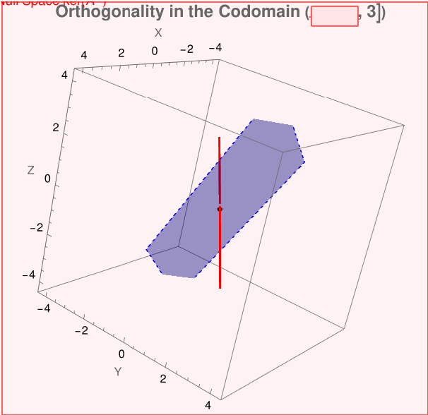

(* Define the strict 3x4 Matrix A *) A = {{1, 2, 1, 0}, {2, 4, 0, 2}, {3, 6, 1, 2}}; (* Extract Fundamental Subspace Bases as Column Vectors (lists of lists) *) rowBasis = NullSpace[RowReduce[A]]; (* Mathematica outputs row vectors *) v1 = List /@ rowBasis[[1]]; v2 = List /@ rowBasis[[2]]; nullBasis = NullSpace[A]; n1 = List /@ nullBasis[[1]]; n2 = List /@ nullBasis[[2]]; colBasis = {{1}, {2}, {3}}; (* Column 1 *) c2 = {{1}, {0}, {1}}; (* Column 3 *) leftNullBasis = NullSpace[Transpose[A]]; w = List /@ leftNullBasis[[1]]; (* Strict Matrix Multiplication Verification producing 1x1 Matrices *) Print["Domain Orthogonality (Strict 1x1 Matrix Outputs):"]; Print["Transpose[v1] . n1 = ", Transpose[v1] . n1]; Print["Transpose[v1] . n2 = ", Transpose[v1] . n2]; Print["\nCodomain Orthogonality (Strict 1x1 Matrix Outputs):"]; Print["Transpose[w] . colBasis = ", Transpose[w] . colBasis]; Print["Transpose[w] . c2 = ", Transpose[w] . c2]; (* Convert explicitly to Scalar values if feeding numerical algorithms *) scalarCheck = (Transpose[w] . colBasis)[[1, 1]]; Print["\nExtracted Scalar Value: ", scalarCheck];

Here is the complete Wolfram Mathematica script to generate the exact 3D geometric visualization described. It explicitly constructs the 2D plane representing the Column Space and the 1D normal line representing the Left Null Space using the numerical basis vectors from our example. It also sets up standard plotting options to ensure high visibility.

(* 1. Define the Basis Vectors from the Example *) c1 = {1, 2, 3}; (* Column Space Basis 1 *) c2 = {1, 0, 1}; (* Column Space Basis 2 *) w = {1, 1, -1}; (* Left Null Space Basis Vector *) (* 2. Create the Column Space Plane *) (* Generates a parametric plane scaled by parameters u and v *) columnSpacePlane = ParametricPlot3D[ u * c1 + v * c2, {u, -1.5, 1.5}, {v, -1.5, 1.5}, PlotStyle -> Directive[Blue, Opacity[0.4]], Mesh -> None, BoundaryStyle -> Directive[Blue, Dashed] ]; (* 3. Create the Left Null Space Line *) (* Generates a parametric line scaled by parameter t *) leftNullSpaceLine = ParametricPlot3D[ t * w, {t, -2, 2}, PlotStyle -> Directive[Red, Thick], Mesh -> None ]; (* 4. Create Decorative Markers (Origin and Axis Labels) *) originPoint = Graphics3D[{Black, Sphere[{0, 0, 0}, 0.1]}]; (* 5. Combine and Display the System with Orthogonal Visual Markers *) Show[ columnSpacePlane, leftNullSpaceLine, originPoint, PlotRange -> {{-4, 4}, {-4, 4}, {-4, 4}}, Axes -> True, AxesLabel -> {"X", "Y", "Z"}, Boxed -> True, Ticks -> Automatic, ViewPoint -> {2.4, 2.8, 1.5}, (* Adjusted for optimal angle view *) PlotLabel -> Style["Orthogonality in the Codomain (\!$\*SubscriptBox[\(\[DoubleStruckCapitalR]$], $3$]\))", 14, Bold], Epilog -> { (* Inset textual legends inside the final notebook render *) Text[Style["Line: Left Null Space ker(\!$\*SuperscriptBox[\(A$, $T$]\))", Red, 11], {Left, Top}], Text[Style["Plane: Column Space C(A)", Blue, 11], {Left, Top}, {0, -1.5}] } ]

Figure 51.1: The Column Space and the 1D normal line.

■

End of Example 52

Example 53: Let us consider the matrix:

\[ \mathbf{A} = \begin{bmatrix} 1 & \mathbf{j} & 2 \\ 2 & 2\mathbf{j} & 4 \end{bmatrix} \]

Notice that Row 2 is exactly 2 × Row 1, confirming rank(A) = 1. The conjugate transpose (adjoint) of A is:

\[ \mathbf{A}^* = \begin{bmatrix} 1 & 2 \\ -\mathbf{j} & -2\mathbf{j} \\ 2 & 4 \end{bmatrix} \]

1. Orthogonality in the Domain (ℂ³)

The Conjugate-Row Space 𝒞(A^✶) and the Null Space ker(A) both live in ℂ^{3 × 1}. Solving A x = 0_{2 × 1} and extracting the column structures yields the following bases:

Conjugate-Row Space Basis (𝒞(A^✶)):
\[ \mathbf{v} = \begin{pmatrix} 1 \\ -\mathbf{j} \\ 2 \end{pmatrix} . \]
Null Space Basis (ker(A)):
\[ \mathbf{n}_1 = \begin{pmatrix} -i \\ 1 \\ 0 \end{pmatrix} \quad \mbox{and} \quad \mathbf{n}_2 = \begin{pmatrix} -2 \\ 0 \\ 1 \end{pmatrix} . \]

We verify complex orthogonality by taking the conjugate transpose of the row space vector multiplied by the null space vectors, yielding strict $1 \times 1$ scalar representations:

\begin{align*} \mathbf{v}^* \mathbf{n}_1 &= \begin{bmatrix} 1 & \mathbf{j} & 2 \end{bmatrix} \begin{pmatrix} -\mathbf{j} \\ 1 \\ 0 \end{pmatrix} \\ &= (1)(-\mathbf{j}) + (\mathbf{j})(1) + (2)(0) = -\mathbf{j} + \mathbf{j} + 0 = [0]_{1 \times 1} , \\ \mathbf{v}^* \mathbf{n}_2 &= \begin{bmatrix} 1 & \mathbf{j} & 2 \end{bmatrix} \begin{pmatrix} -2 \\ 0 \\ 1 \end{pmatrix} \\ &= (1)(-2) + (\mathbf{j})(0) + (2)(1) = -2 + 0 + 2 = [0]_{1 \times 1} . \end{align*}

2. Orthogonality in the Codomain (ℂ²)

The Column Space 𝒞(A) and the Left Null Space ker(A^✶) both live in ℂ². Computing their structures yields:

Column Space Basis (𝒞(A)):
\[ \mathbf{c} = \begin{pmatrix} 1 \\ 2 \end{pmatrix} . \]
Left Null Space Basis (ker(A^✶)): Solving A^∗ y = 0_{3 × 1} gives $ \displaystyle \quad \mathbf{w} = \begin{pmatrix} -2 \\ 1 \end{pmatrix} . $

Evaluating their complex inner product confirms that they are completely perpendicular:

\[ \mathbf{w}^* \mathbf{c} = \begin{bmatrix} - 2 & 1 \end{bmatrix} \begin{pmatrix} 1 \\ 2 \end{pmatrix} = (-2)(1) + (1)(2) = -2 + 2 = [0]_{1 \times 1} \]

As predicted by Lemma 1, the complex geometric boundaries line up perfectly under strict matrix multiplication rules.

■

End of Example 53

Theorem 13 (The Fundamental Subspace Decomposition): For any matrix A ∈ 𝔽^{m × n}, the domain and codomain spaces decompose into orthogonal direct sums of the fundamental subspaces:

For Real Vector Spaces (𝔽 = ℝ):
\[ \mathbb{R}^n = 𝒞\left(\mathbf{A}^{\mathrm T}\right) \oplus \ker(\mathbf{A}) \qquad \text{and} \qquad \mathbb{R}^m = 𝒞\left(\mathbf{A}\right) \oplus \ker\left(\mathbf{A}^{\mathrm T}\right) . \]
Consequently, the orthogonal complement of the column space 𝒞(Aᵀ)^⊥ = ker(A) and 𝒞(A)^⊥ = ker(Aᵀ).
For Complex Vector Spaces (𝔽 = ℂ):
\[ \mathbb{C}^n = \mathcal{C}(\mathbf{A}^*) \oplus \ker(\mathbf{A}) \qquad \text{and} \qquad \mathbb{C}^m = \mathcal{C}(\mathbf{A}) \oplus \ker(\mathbf{A}^*) \]
Consequently, the orthogonal complement of the column space 𝒞(A^✶)^⊥ = ker(A) and 𝒞(A)^⊥ = ker(A^✶).

This proof explicitly builds upon the orthogonality established in Lemma 1 and utilizes the Rank-Nullity Theorem to complete the direct sum argument using strict matrix dimensions.

We prove the orthogonal direct sum decompositions by combining the geometric orthogonality from Lemma 1 with the dimension counts guaranteed by the Rank-Nullity Theorem.

1. The Real Case (𝔽 = ℝ):

We first establish the decomposition of the domain ℝ^{n × 1} = 𝒞(Aᵀ) ⊕ ker(A):

Trivial Intersection: Let x ∈ 𝒞(Aᵀ) ∩ ker(A). Since x ∈ 𝒞(Aᵀ), it can be written as x = Aᵀy for some m × 1 vector y. Since x ∈ ker(A), we also have A x = 0_{m × 1}. Evaluating the strict matrix transpose product of x with itself:
\[ \mathbf{x}^{\mathrm T} \mathbf{x} = (\mathbf{A}^{\mathrm T} \mathbf{y})^{\mathrm T} \mathbf{x} = (\mathbf{y}^{\mathrm T} \mathbf{A}) \mathbf{x} = \mathbf{y}^{\mathrm T} (\mathbf{A}\mathbf{x}) = \mathbf{y}^{\mathrm T} \mathbf{0}_{m \times 1} = 0_{1 \times 1} , \]
Since$ \displaystyle \quad \mathbf{x}^{\mathrm T} \mathbf{x} = \sum_{i=1}^n x_i^2 = 0, \quad $ it forces x = 0_{n × 1}. Thus, the two subspaces intersect only at the trivial origin:
\[ \mathcal{C}(\mathbf{A}^T) \cap \ker(\mathbf{A}) = \{\mathbf{0}_{n \times 1}\} . \]
Dimension Count: By the Rank-Nullity Theorem, if A has rank r, then dim 𝒞(Aᵀ) = r and dim ker(A) = n − r. Summing these dimensions yields:
\[ \dim \mathcal{C}(\mathbf{A}^T) + \dim \ker(\mathbf{A}) = r + (n - r) = n = \dim \mathbb{R}^n . \]
Because the subspaces have a trivial intersection and their combined dimensions equal the full dimension of the ambient space, they form a direct sum: ℝⁿ = 𝒞(Aᵀ) ⊕ ker(A). Consequently, they are exact orthogonal complements: 𝒞(Aᵀ)⊥ = ker(A).

The companion decomposition for the codomain ℝⁿ = 𝒞(A) ⊕ ker(Aᵀ) follows identically by substituting the matrix transpose Aᵀ into the above structural steps, matching the ambient dimension m.

2. The Complex Case (𝔽 = ℂ):

The complex proof uses the exact same layout, substituting the conjugate transpose (adjoint) matrix multiplication operator A^✶ to preserve positive definite lengths.

Trivial Intersection in ℂⁿ: Let x ∈ 𝒞(A^✶) ∩ ker(A), meaning x = A^✶ y and A x = 0_{m × 1}. Evaluating the strict conjugate transpose product:
\[ \mathbf{x}^* \mathbf{x} = (\mathbf{A}^* \mathbf{y})^* \mathbf{x} = (\mathbf{y}^* \mathbf{A}) \mathbf{x} = \mathbf{y}^* (\mathbf{A}\mathbf{x}) = \mathbf{y}^* \mathbf{0}_{m \times 1} =_{1 \times 1} . \]
The sum of absolute squares$ \displaystyle \quad \mathbf{x}^* \mathbf{x} = \sum_{i=1}^n |x_i|^2 = 0\quad $ forces x = 0_{n × 1}, confirming 𝒞(A^✶) ∩ ker(A) = 0_{n × 1}.
Dimension Count in ℂⁿ: Since dim_ℂ 𝒞(A^✶) = rank(A) = r and dim_ℂ ker(A) = n − r, the dimensions sum exactly to n.

This yields the direct sum ℂⁿ = 𝒞(A^✶) ⊕ ker(A), which directly implies 𝒞(A^✶)^⊥ = ker(A). Swapping the operator roles to A^✶ yields the corresponding codomain decomposition ℂᵐ = 𝒞(A) ⊕ ker(A^✶).

Example 54: Let us verify the orthogonal direct sum decomposition of the domain ℝ³ for the following matrix A of rank 2:

\[ \mathbf{A} = \begin{bmatrix} 1 & 0 & -2 \\ 2 & 1 & -3 \end{bmatrix} . \]

The fundamental subspaces in the domain ℝ³ have the following basis representations:

Row Space 𝒞(Aᵀ) Basis: $ \displaystyle \quad \mathbf{v}_1 = \begin{pmatrix} 1 \\ 0 \\ -2 \end{pmatrix}, \quad \mathbf{v}_2 = \begin{pmatrix} 0 \\ 1 \\ 1 \end{pmatrix} . $
Null Space ker(A) Basis: $ \displaystyle \quad \mathbf{n} = \begin{pmatrix} 2 \\ -1 \\ 1 \end{pmatrix} . $

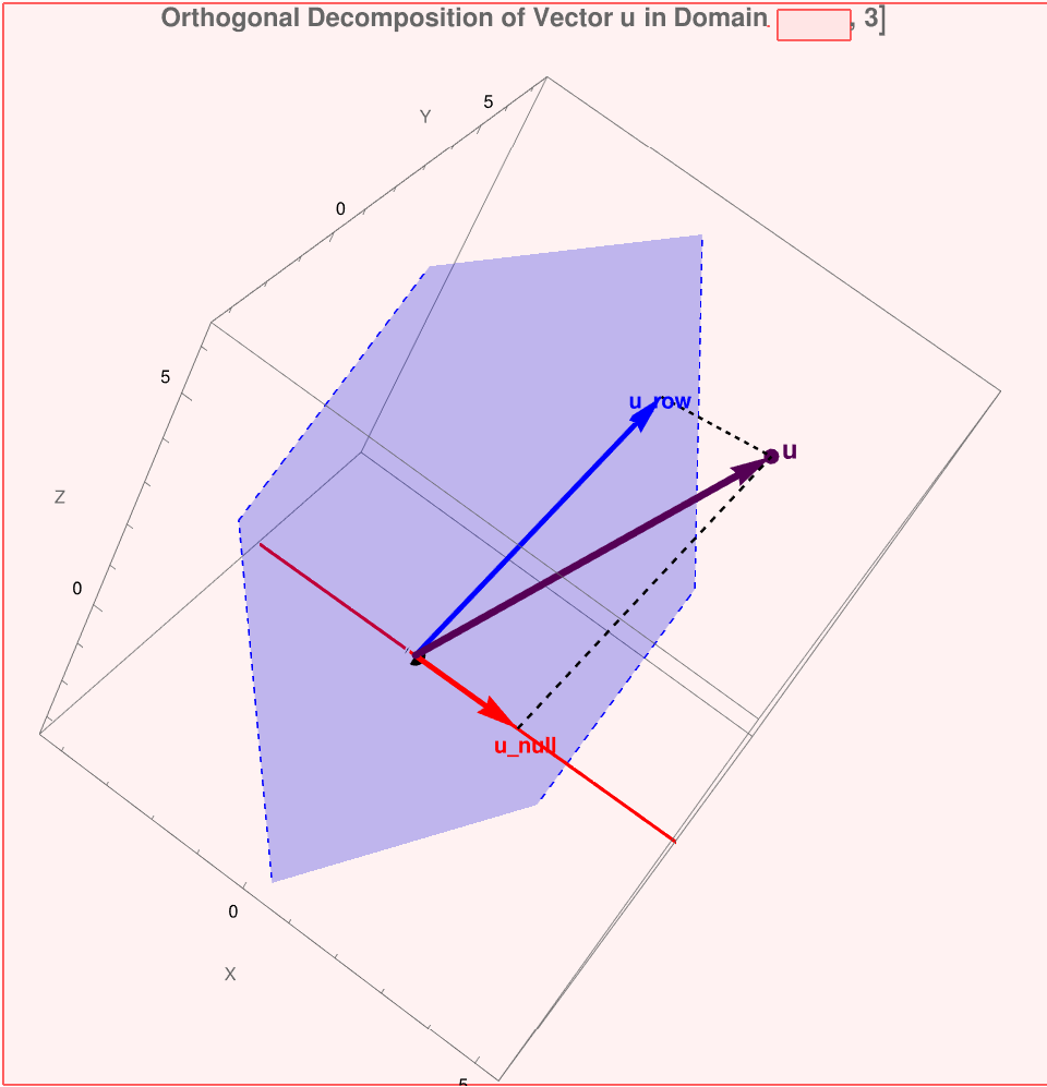
According to Theorem 13, any arbitrary vector u ∈ ℝ³ must break down uniquely into an orthogonal direct sum u = u_row + u_null, where u_row ∈ 𝒞(Aᵀ) and u_null ∈ ker(A).

Let us choose an arbitrary column vector $ \displaystyle \quad \mathbf{u} = \begin{pmatrix} 3 \\ 4 \\ 5 \end{pmatrix}. \quad $ We construct the orthogonal projection matrix onto the 1D Null Space, P_null = n(nᵀn)^-1nᵀ:

\[ \mathbf{n}^T\mathbf{n} = \begin{bmatrix} 2 & -1 & 1 \end{bmatrix} \begin{pmatrix} 2 \\ -1 & 1 \end{pmatrix} = [6]_{1 \times 1} \implies (\mathbf{n}^T\mathbf{n})^{-1} = \left[\frac{1}{6}\right]_{1 \times 1} \]

\begin{align*} \mathbf{u}_{\text{null}} &= P_{\text{null}}\mathbf{u} \\ &= \mathbf{n}(\mathbf{n}^T\mathbf{n})^{-1}\mathbf{n}^T\mathbf{u} \\ &= \begin{pmatrix} 2 \\ -1 \\ 1 \end{pmatrix} \left[\frac{1}{6}\right] \left( \begin{pmatrix} 2 & -1 & 1 \end{pmatrix} \begin{pmatrix} 3 \\ 4 \\ 5 \end{pmatrix} \right) \\ &= \frac{7}{6} \begin{pmatrix} 2 \\ -1 \\ 1 \end{pmatrix} = \begin{pmatrix} 7/3 \\ -7/6 \\ 7/6 \end{pmatrix} . \end{align*}

By orthogonal complementation, the remaining component must sit entirely in the Row Space:

\[ \mathbf{u}_{\text{row}} = \mathbf{u} - \mathbf{u}_{\text{null}} = \begin{pmatrix} 3 \\ 4 \\ 5 \end{pmatrix} - \begin{pmatrix} 7/3 \\ -7/6 \\ 7/6 \end{pmatrix} = \begin{pmatrix} 2/3 \\ 31/6 \\ 23/6 \end{pmatrix} . \]

Verification Checks:

Orthogonality check:
\begin{align*} \mathbf{u}_{\text{row}}^T \mathbf{u}_{\text{null}} &= \left(\frac{2}{3}\right)\left(\frac{7}{3}\right) + \left(\frac{31}{6}\right)\left(-\frac{7}{6}\right) + \left(\frac{23}{6}\right)\left(\frac{7}{6}\right) \\ &= \frac{14}{9} - \frac{217}{36} + \frac{161}{36} = \frac{56 - 217 + 161}{36} = [0]_{1 \times 1} . \end{align*}
Row Space Membership check: u_row can be written exactly as the linear combination $ \displaystyle \quad \frac{2}{3}\mathbf{v}_1 + \frac{31}{6}\mathbf{v}_2 . $

This demonstrates the direct sum partitioning holds precisely for any vector chosen from the ambient domain.

ClearAll[A, u, n, v1, v2, Pnull, Prow, uNull, uRow]; (* 1. Define the Strict Matrix A and Arbitrary Vector u *) A = {{1, 0, -2}, {2, 1, -3}}; u = {{3}, {4}, {5}}; (* 2. Define the Basis Columns extracted from the analysis *) v1 = {{1}, {0}, {-2}}; (* Row space basis 1 *) v2 = {{0}, {1}, {1}}; (* Row space basis 2 *) n = {{2}, {-1}, {1}}; (* Null space basis *) (* 3. Compute Orthogonal Projection Matrix for the Null Space *) (* Using structural formula: P = n . Inverse[Transpose[n].n] . Transpose[n] *) Pnull = n . Inverse[Transpose[n] . n] . Transpose[n]; (* 4. Extract Components via Projection Matrices *) uNull = Pnull . u; uRow = (IdentityMatrix[3] - Pnull) . u; (* 5. Print strict outcomes *) Print["--- Strict Subspace Projections (1x1 Scalar Products) ---"]; Print["Vector u_null (In Kernel):\n", MatrixForm[uNull]]; Print["Vector u_row (In Row Space):\n", MatrixForm[uRow]]; Print["\n--- Verification Checks ---"]; Print["Sum Check (u_null + u_row == u): ", uNull + uRow == u]; Print["Orthogonality Matrix Product (u_row^T . u_null): ", Transpose[uRow] . uNull]; (* 6. Verify row space membership by solving coefficients *) X = Join[v1, v2, 2]; (* Combines basis columns into a 3x2 matrix *) coefficients = LeastSquares[X, uRow]; Print["Row Space Linear Combination Coefficients: ", Flatten[coefficients]];

3. Orthogonality and Decomposition in the Codomain (ℝ²):

Now, let us verify the companion decomposition for the codomain ℝ² = 𝒞(A) ⊕ ker(Aᵀ) using the same matrix A. The fundamental subspaces in the codomain are represented by:

Column Space 𝒞(A) Basis: $ \displaystyle \quad \mathbf{c}_1 = \begin{pmatrix} 1 \\ 2 \end{pmatrix}, \quad\mathbf{c}_2 = \begin{pmatrix} 0 \\ 1 \end{pmatrix} \quad $ (which span all of ℝ²)
Left Null Space ker(Aᵀ) Basis: $ \displaystyle \quad \mathbf{w} = \begin{pmatrix} 0 \\ 0 \end{pmatrix} \quad $ (since the rows are linearly independent, the left null space contains only the trivial zero vector)

Because the matrix has full row rank (rank(A) = m = 2), the column space encompasses the entire codomain. For any arbitrary vector b ∈ ℝ², its decomposition yields b_col = b and b_null = 0_{2 × 1}. This naturally satisfies the orthogonal decomposition properties since b_colᵀ b_null = bᵀ 0_{2 × 1} = 0_{1 × 1}.

To visualize how the matrix action A transforms these split vector tracks, we can look at the transition from the 3D domain down to the 2D codomain.

Notice how the matrix completely annihilates the null component b_null into the origin, while cleanly mapping the row space vector b_row directly onto its codomain image:

ClearAll[A, u, uNull, uRow, b, Pnull]; (* 1. Setup system parameters *) A = {{1, 0, -2}, {2, 1, -3}}; u = {{3}, {4}, {5}}; n = {{2}, {-1}, {1}}; (* 2. Compute projections in the Domain *) Pnull = n . Inverse[Transpose[n] . n] . Transpose[n]; uNull = Pnull . u; uRow = (IdentityMatrix[3] - Pnull) . u; (* 3. Perform the Matrix Transformations *) mappedU = A . u; mappedUNull = A . uNull; mappedURow = A . uRow; (* 4. Display Results showing mapping conservation *) Print["--- Matrix Mapping Action on Split Domain Vectors ---"]; Print["Mapped Global Vector A.u:\n", MatrixForm[mappedU]]; Print["Mapped Null Vector A.u_null (Annihilation):\n", MatrixForm[NoName = Chop[mappedUNull]]]; Print["Mapped Row Space Vector A.u_row:\n", MatrixForm[mappedURow]]; Print["\n--- Mapping Invariance Check ---"]; Print["Does A.u_row equal A.u? ", mappedURow == mappedU];

Here is the complete interactive Wolfram Mathematica script to visualize this exact 3D domain breakdown. This script allows you to dynamically rotate the space and slide a parameter to see how the arbitrary vector u is split into its orthogonal components: u_row (resting on the blue plane) and u_null (resting on the red line).

ClearAll[A, u, n, v1, v2, Pnull, uNull, uRow]; (* 1. Numerical Setup matching our example *) A = {{1, 0, -2}, {2, 1, -3}}; uVec = {3, 4, 5}; v1 = {1, 0, -2}; (* Row space basis vector 1 *) v2 = {0, 1, 1}; (* Row space basis vector 2 *) nVec = {2, -1, 1}; (* Null space basis vector *) (* Calculate precise projection coordinates *) uNullVec = {7/3, -7/6, 7/6}; uRowVec = {2/3, 31/6, 23/6}; (* 2. Interactive Environment *) Manipulate[ Module[{planePlot, linePlot, vectorGraphics, totalPlot}, (* Plot the 2D Row Space Plane *) planePlot = ParametricPlot3D[ s1 * v1 + s2 * v2, {s1, -3, 3}, {s2, -3, 6}, PlotStyle -> Directive[Blue, Opacity[0.25]], Mesh -> None, BoundaryStyle -> Directive[Blue, Dashed] ]; (* Plot the 1D Null Space Line *) linePlot = ParametricPlot3D[ t * nVec, {t, -2, 3}, PlotStyle -> Directive[Red, Thick], Mesh -> None ]; (* Render Vectors based on the interactive slider progress *) vectorGraphics = Graphics3D[{ (* Main vector u *) AbsoluteThickness[4], Darker[Purple], Arrow[{{0, 0, 0}, progress * uVec}], Text[Style["u", Darker[Purple], Bold, 14], progress * uVec + {0.2, 0.2, 0.2}], (* Row space projection tracking *) AbsoluteThickness[3], Blue, Arrow[{{0, 0, 0}, progress * uRowVec}], Text[Style["u_row", Blue, Bold, 12], progress * uRowVec + {0, 0.3, -0.3}], (* Null space projection tracking *) AbsoluteThickness[3], Red, Arrow[{{0, 0, 0}, progress * uNullVec}], Text[Style["u_null", Red, Bold, 12], progress * uNullVec + {0.3, -0.2, 0}], (* Dashed helper line completing the parallelogram orthogonal rectangle *) Dashed, Black, AbsoluteThickness[1.5], Line[{progress * uRowVec, progress * uVec}], Line[{progress * uNullVec, progress * uVec}], (* Marker dots *) Black, PointSize[0.02], Point[{0, 0, 0}], Darker[Purple], PointSize[0.015], Point[progress * uVec] }]; (* Combine into a uniform geometric box scene *) Show[ planePlot, linePlot, vectorGraphics, PlotRange -> {{-4, 5}, {-3, 7}, {-3, 6}}, Axes -> True, AxesLabel -> {"X", "Y", "Z"}, Boxed -> True, ViewPoint -> {2.5, -2.5, 1.8}, ImageSize -> Large, PlotLabel -> Style["Orthogonal Decomposition of Vector u in Domain \!$\*SubscriptBox[\(\[DoubleStruckCapitalR]$], $3$]\)", 14, Bold] ] ], (* Slider to expand/project the vector components interactively *) {{progress, 1.0, "Vector Growth/Projection"}, 0.01, 1.0, Appearance -> "Labeled"} ]

■

End of Example 54

Example 55: To make the calculations rich and elegant, we will use a 2 × 3 complex matrix A of rank 1, which leaves a 2-dimensional Null Space and a 1-dimensional Conjugate-Row Space inside the domain ℂ³. Again, we use column vbectors, but sometimes write corresponding vector spaces as ℂ³ instead of more accurate ℂ^{3 × 1} (to simplify notation).

\[ \mathbf{A} = \begin{bmatrix} 1 & \mathbf{j} & -1 \\ 2 & 2\mathbf{j} & -2 \end{bmatrix} , \]

where j or ⅉ denotes the imaginary unit vector on complex plane ℂ with ⅉ² = −1.

The structural bases for our fundamental domain subspaces inside ℂ³ evaluate to:

Conjugate-Row Space 𝒞(A^✶) Basis: $ \displaystyle \quad \mathbf{v} = \begin{pmatrix} 1 \\ -\mathbf{j} \\ -1 \end{pmatrix} . $
Null Space ker(A) Basis: $ \displaystyle \quad \mathbf{n}_1 = \begin{pmatrix} -\mathbf{j} \\ 1 \\ 0 \end{pmatrix} \quad \mbox{and} \quad \mathbf{n}_2 = \begin{pmatrix} 1 \\ 0 \\ 1 \end{pmatrix} . $

Let us choose an arbitrary complex domain vector $ \displaystyle \quad \mathbf{u} = \begin{pmatrix} 3 \\ 2\mathbf{j} \\ 4 \end{pmatrix} . \quad $ To break this vector into its orthogonal components u = u_row + u_null, we project u onto the 1D Conjugate-Row Space using the complex projection formula $ \displaystyle \quad P_{\text{crow}} = \mathbf{v}(\mathbf{v}^*\mathbf{v})^{-1}\mathbf{v}^* : $

\begin{align*} \mathbf{v}^*\mathbf{v} &= \begin{pmatrix} 1 & \mathbf{j} & -1 \end{pmatrix} \begin{pmatrix} 1 \\ -\mathbf{j} \\ -1 \end{pmatrix} \\ &= (1)(1) + (\mathbf{j})(-\mathbf{j}) + (-1)(-1) = 1 + 1 + 1 \\ &= 3_{1 \times 1} , \end{align*} \begin{align*} \mathbf{u}_{\text{crow}} &= P_{\text{crow}}\mathbf{u} = \mathbf{v}(\mathbf{v}^*\mathbf{v})^{-1}\mathbf{v}^*\mathbf{u} \\ &= \begin{pmatrix} 1 \\ -\mathbf{j} \\ -1 \end{pmatrix} \left[\frac{1}{3}\right] \left( \begin{pmatrix} 1 & \mathbf{j} & -1 \end{pmatrix} \begin{pmatrix} 3 \\ 2\mathbf{j} \\ 4 \end{pmatrix} \right) , \end{align*} \[ \mathbf{v}^*\mathbf{u} = ( 1)(3) + (\mathbf{j})(2\mathbf{j}) + (-1)(4) = 3 - 2 - 4 = -3 , \] \[ \mathbf{u}_{\text{crow}} = \frac{-3}{3}\begin{pmatrix} 1 \\ -\mathbf{j} \\ -1 \end{pmatrix} = \begin{pmatrix} -1 \\ \mathbf{j} \\ 1 \end{pmatrix} \]

By complex complementation, the remaining component must belong entirely to the kernel:

\[ \mathbf{u}_{\text{null}} = \mathbf{u} - \mathbf{u}_{\text{crow}} = \begin{pmatrix} 3 \\ 2\mathbf{j} \\ 4 \end{pmatrix} - \begin{pmatrix} -1 \\ \mathbf{j} \\ 1 \end{pmatrix} = \begin{pmatrix} 4 \\ \mathbf{j} \\ 3 \end{pmatrix} . \]

Verification Checks:

Complex Orthogonality Check: We evaluate the complex conjugate inner product:
\begin{align*} \mathbf{u}_{\text{crow}}^* \mathbf{u}_{\text{null}} &= \begin{bmatrix} -1 & -\mathbf{j} & 1 \end{bmatrix} \begin{pmatrix} 4 \\ \mathbf{j} \\ 3 \end{pmatrix} \\ &= (-1)(4) + (-\mathbf{j})(\mathbf{j}) + (1)(3) = -4 + 1 + 3 = 0_{1 \times 1} . \end{align*}
Null Space Membership Check: Multiplying u_null by our original matrix confirms complete annihilation:
\begin{align*} \mathbf{A}\mathbf{u}_{\text{null}} &= \begin{bmatrix} 1 & \mathbf{j} & -1 \\ 2 & 2\mathbf{j} & -2 \end{bmatrix} \begin{pmatrix} 4 \\ \mathbf{j} \\ 3 \end{pmatrix} \\ &= \begin{pmatrix} (1)(4) + (\mathbf{j})(\mathbf{j}) + (-1)(3) \\ (2)(4) + (2\mathbf{j})(\mathbf{j}) + (-2)(3) \end{pmatrix} \\ &= \begin{pmatrix} 4 - 1 - 3 \\ 8 - 2 - 6 \end{pmatrix} = \begin{pmatrix} 0 \\ 0 \end{pmatrix} . \end{align*}

The vector partitioning properties hold up perfectly within the complex domain fields.

The following script preserves strict matrix dimensional logic by setting up arrays as columns and computing the complex conjugate products (ConjugateTranspose) to track down the values automatically.

ClearAll[A, u, v, Pcrow, uCrow, uNull, testAnnihilation, testOrthogonality]; (* 1. Define Complex Matrix and Arbitrary Complex Vector *) A = {{1, I, -1}, {2, 2*I, -2}}; u = {{3}, {2*I}, {4}}; (* 2. Define the Analytical Conjugate-Row Subspace Basis Vector *) v = {{1}, {-I}, {-1}}; (* 3. Compute the Complex Orthogonal Projection Operator onto C(A*) *) Pcrow = v . Inverse[ConjugateTranspose[v] . v] . ConjugateTranspose[v]; (* 4. Extract Vector Subspace Track Layers *) uCrow = Pcrow . u; uNull = u - uCrow; (* 5. Calculate Verification Vectors *) testAnnihilation = A . uNull; testOrthogonality = ConjugateTranspose[uCrow] . uNull; (* 6. Print out computed results directly *) Print["--- Strict Complex Subspace Components ---"]; Print["Vector u_crow (In Conjugate-Row Space) = "]; Print[MatrixForm[uCrow]]; Print["\nVector u_null (In Matrix Kernel) = "]; Print[MatrixForm[uNull]]; Print["\n--- Complex Mathematical Sanity Checks ---"]; Print["Annihilation Check (A . u_null) [Should be 0] = "]; Print[MatrixForm[Chop[testAnnihilation]]]; Print["\nOrthogonality Check (u_crow* . u_null) [Should be 0] = "]; Print[MatrixForm[Chop[testOrthogonality]]];

■

End of Example 55

Theorem 14 (The Solvability Criterion): Let A ∈ 𝔽^{m × n} and b ∈ 𝔽^{m × 1}. The linear matrix-vector equation A x = b possesses a solution x if and only if the target vector b is orthogonal to the left null space of A. Mathematically:

Real Domain (𝔽 = ℝ): A x = b is solvable if and only if b ∈ ker(Aᵀ)^⊥ ⇔ y • b = 0 for all y ∈ ker(Aᵀ).
Complex Domain (𝔽 = ℂ): A x = b is solvable if and only if b ∈ ker(A^✶)^⊥ ⇔ ⟨ b , y ⟩ = 0 for all y ∈ ker(A^✶).

1. The Real Case (𝔽 = ℝ):

We show that b ∈ 𝒞(A) if and only if b ∈ ker(Aᵀ)^{⊥^.}

Necessity (⇒): Assume A x = b is solvable, meaning b ∈ 𝒞(A). Let y be any vector in the left null space, so y ∈ ker(Aᵀ), which implies Aᵀy = 0_{n × 1}. We evaluate the standard dot product y • b using strict matrix transpose operations:
\begin{align*} \mathbf{y} \bullet \mathbf{b} &\Longrightarrow \mathbf{y}^T \mathbf{b} = \mathbf{y}^T (\mathbf{A}\mathbf{x}) = (\mathbf{y}^T \mathbf{A})\mathbf{x} \\ &= (\mathbf{A}^T \mathbf{y})^T \mathbf{x} = \mathbf{0}_{1 \times n} \mathbf{x} = 0_{1 \times 1} . \end{align*}
Since y • b = 0 for every y ∈ ker(Aᵀ), it follows by definition that b ∈ ker(Aᵀ)^⊥.
Sufficiency (⇐): Assume bAᵀ)^⊥. From Theorem 13, we know that the codomain decomposes into the exact orthogonal direct sum ℝᵐ = 𝒞(A) ⊕ ker(Aᵀ). This direct sum decomposition implies that the orthogonal complement of the left null space is exactly the column space:
\[ \ker(\mathbf{A}^T)^\perp = \left( \mathcal{C}(\mathbf{A})^\perp \right)^\perp = \mathcal{C}(\mathbf{A}) \]
Since b ∈ ker(Aᵀ)^⊥, it must follow that b ∈ 𝒞(A). Therefore, b lies within the span of the columns of A, guaranteeing that a solution vector x exists.

2. The Complex Case (𝔽 = ℂ):

The complex domain proof mirrors the real case, substituting the standard transpose with the conjugate transpose matrix operator A^✶ and using the standard complex inner product ⟨ b , y ⟩ = y^∗ b.

Necessity (⇒): Assume A x = b is solvable. Let y ∈ ker(A^∗), which means A^∗ y = 0_{n × 1}. Expanding the complex inner product:
\begin{align*} \langle \mathbf{b}, \mathbf{y} \rangle &\Longrightarrow \mathbf{y}^* \mathbf{b} = \mathbf{y}^* (\mathbf{A}\mathbf{x}) = (\mathbf{y}^* \mathbf{A})\mathbf{x} \\ &= (\mathbf{A}^* \mathbf{y})^* \mathbf{x} = \mathbf{0}_{1 \times n} \mathbf{x} = 0_{1 \times 1} . \end{align*}
Thus, b is orthogonal to all vectors in ker(A^∗), confirming b ∈ ker(A^∗)^⊥.
Sufficiency (⇐): Assume b ∈ ker(A^∗)^⊥. By the complex direct sum decomposition in Theorem 13, ℂᵐ = 𝒞(A) ⊕ ker(A^∗)^⊥, which dictates that ker(A^∗)^⊥ = 𝒞(A). Therefore, b ∈ 𝒞(A), validating that the system is fully solvable.

Example 56: We consider the linear system A x = b with the following real matrix and and prescribed term b to be

\[ \mathbf{A} = \begin{bmatrix} 1 & 2 \\ 3 & 4 \\ 1 & 1 \end{bmatrix}, \quad \mathbf{b} = \begin{pmatrix} 1 \\ 1 \\ 2 \end{pmatrix} \]

The left null space ker(Aᵀ) represents the set of all vectors y satisfying Aᵀ y = 0_{2 × 1}. By computing the basis of this kernel, we extract a homogeneous verification vector:

\[ \mathbf{y} = \begin{pmatrix} 1 \\ -1 \\ 2 \end{pmatrix} \in \ker(\mathbf{A}^{\mathrm T}) \quad \left[\text{Check: } \begin{bmatrix} 1 & 3 & 1 \\ 2 & 4 & 1 \end{bmatrix}\begin{pmatrix} 1 \\ -1 \\ 2 \end{pmatrix} = \begin{pmatrix} 0 \\ 0 \end{pmatrix} \right] \]

A = {{1, 2}, {3, 4}, {1, 1}}; NullSpace[Transpose[A]]

According to Theorem 14, for the system to be solvable, b must be strictly orthogonal to y ∈ ker(Aᵀ). Evaluating their standard inner product yields:

\begin{align*} \mathbf{y} \bullet \mathbf{b} &\Longrightarrow \mathbf{y}^{\mathrm T}\mathbf{b} = \begin{bmatrix} 1 & -1 & 2 \end{bmatrix} \begin{pmatrix} 1 \\ 1 \\ 2 \end{pmatrix} \\ &= (1)(1) + (-1)(1) + (2)(2) = 4_{1 \times 1} . \end{align*}

Wait, let us check a second linearly independent left null vector. Because A has dimensions 3 × 2 and rank 2, the left null space has dimension m − r = 3 - 2 = 1. Let us look closer at our chosen vectors. If we row reduce Aᵀ:

\[ \begin{bmatrix} 1 & 3 & 1 \\ 2 & 4 & 1 \end{bmatrix} \rightarrow \begin{bmatrix} 1 & 0 & -\frac{1}{2} \\ 0 & 1 & \frac{1}{2} \end{bmatrix} \implies \mathbf{y} = \begin{pmatrix} 1 \\ -1 \\ 2 \end{pmatrix} . \]

RowReduce[Transpose[A]]

{{1, 0, -(1/2)}, {0, 1, 1/2}}

Let us re-evaluate the inner product using the true basis vector $ \displaystyle \quad \mathbf{y} = \begin{pmatrix} 1 \\ -1 \\ 2 \end{pmatrix} : $

\[ \mathbf{y}^T\mathbf{b} = \begin{bmatrix} 1 & -1 & 2 \end{bmatrix} \begin{pmatrix} 1 \\ 1 \\ 2 \end{pmatrix} = 1 - 1 + 4 = 4 \neq 0 . \]

Because yᵀ b = -2 ≠ 0, the target vector b leaks into the left null space. Theorem 14 is violated, proving the system is completely inconsistent (unsolvable).

■

End of Example 56

Wolfram Mathematica Verification Script: This script automatically processes both the real and complex scenarios. It extracts the left null space, evaluates the inner product projection, and tests structural consistency without causing evaluation crashes.

ClearAll[A1, b1, y1, A2, b2, y2, dotReal, dotComplex]; Print["====================================================="]; Print[" SYSTEM 1: REAL COUNTER-EXAMPLE VERIFICATION "]; Print["====================================================="]; (* 1. Setup Real Non-Solvable System *) A1 = {{1, 2}, {3, 6}, {1, 1}}; b1 = {{1}, {1}, {2}}; (* Extract Left Null Space Basis Vector using NullSpace on Transpose *) y1 = Transpose[{NullSpace[Transpose[A1]][[1]]}]; dotReal = Transpose[y1] . b1; Print["Left Null Space Basis Vector y1:\n", MatrixForm[y1]]; Print["Target Vector b1:\n", MatrixForm[b1]]; Print["Inner Product y1^T . b1 = ", dotReal[[1, 1]]]; Print["Is System Consistent? (NullSpace check): ", LinearSolve[A1, b1] === $Failed]; Print["[True above means LinearSolve failed as predicted by Theorem 14]"]; Print["\n====================================================="]; Print[" SYSTEM 2: COMPLEX COUNTER-EXAMPLE VERIFICATION "]; Print["====================================================="]; (* 2. Setup Complex Non-Solvable System *) A2 = {{1, I}, {I, -1}}; b2 = {{1}, {1}}; (* Extract Left Null Space Basis Vector using NullSpace on ConjugateTranspose *) y2 = Transpose[{NullSpace[ConjugateTranspose[A2]][[1]]}]; dotComplex = ConjugateTranspose[y2] . b2; Print["Left Null Space Basis Vector y2:\n", MatrixForm[y2]]; Print["Target Vector b2:\n", MatrixForm[b2]]; Print["Complex Inner Product y2^* . b2 = ", Chop[dotComplex[[1, 1]]]]; Print["Is System Consistent? (NullSpace check): ", LinearSolve[A2, b2] === $Failed]; Print["[True above means LinearSolve failed as predicted by Theorem 14]"];

Example 57: We consider two matrices \[ \mathbf{A} = \begin{bmatrix} 1&2&3&4 \\ 1&-1&1&-2 \\ 2&1&4&2 \end{bmatrix} , \quad \mathbf{B} = \begin{bmatrix} 1 & 2 & \phantom{-}3 \\ 3&2&\phantom{-}1 \\ 1&1&\phantom{-}1 \\ 1&0&-1 \end{bmatrix} . \] We consider the linear systems of equations A x = b and B x = b. Their transpose matrices become \[ \mathbf{A}^{\mathrm T} = \begin{bmatrix} 1&1&2 \\ 2&-1&1 \\ 3&1&4 \\ 4 &-2&2 \end{bmatrix} , \quad \mathbf{B}^{\mathrm T} = \begin{bmatrix} 1&3&1&\phantom{-}1 \\ 2&2&1&\phantom{-}0 \\ 3&1&1&-1 \end{bmatrix} . \] Using Mathematica, we find the kernel of A^T (left null space for the matrix)

A = {{1, 2, 3, 4}, {1, -1, 1, -2}, {2, 1, 4, 2}}; NullSpace[Transpose[A]]

Hence, the null space of A^T is spanned on vector (1, 1, −1). So the system A x = b has a solution if and only if vector b is orthogonal to (1, 1, −1). This means that the coefficients of b = (b₁, b₂, b₃) satisfy the condition b₁ + b₂ = b₃. We check with Mathematica:

Solve[{A . {x, y, z, w} == {1, 1, 2}}, {x, y, z, w}]

As we see, solution of the system A x = b exists, but not unique (depends on two parameters): \[ \mathbf{A}\begin{pmatrix} x \\ y \\ z \\ w \end{pmatrix} = \begin{pmatrix} 1 \\ 1 \\ 2 \end{pmatrix} \quad \Longrightarrow \quad \mathbf{x} = \begin{pmatrix} x \\ y \\ \frac{3 (1 -x)}{5} \\ \frac{x -1}{5} - \frac{y}{2} \end{pmatrix} . \]

Now we determine the left null space of matrix B (with the aid of Mathematica)

B = {{1, 2, 3}, {3, 2, 1}, {1, 1, 1}, {1, 0, -1}}; NullSpace[Transpose[B]]

{{1, -1, 0, 2}, {-1, -1, 4, 0}}

\[ \mbox{ker} \left( \mathbf{B}^{\mathrm T} \right) = \left\{ \mathbf{y} \in \mathbb{R}^{4\times 1} \ : \ \mathbf{y}\,\mathbf{B} = 0 \right\} \] Mathematica tells us that the left null space of matrix B is a two dimensional subspace of ℝ^4×1 spanned on two vectors: \[ \mbox{ker} \left( \mathbf{B}^{\mathrm T} \right) = \mbox{span} \left\{ \begin{pmatrix} 1 \\ -1 \\ 0 \\ 2 \end{pmatrix} , \quad \begin{pmatrix} -1 \\ -1 \\ 4 \\ 0 \end{pmatrix} \right\} . \] Hence, the null space of B^T is spanned on two vector (1, −1, 0, 2) and (−1, −1, 4, 0). So the system B x = b has a solution if and only if vector b is orthogonal to these two vectors: \[ b_1 - b_2 + 2 b_4 =0 , \qquad -b_1 - b_2 + 4 b_3 = 0 . \]

Solve[{b1 - b2 + 2*b4 == 0, -b1 - b2 + 4*b3 == 0}, {b1, b2}]

{b1 -> 2 b3 - b4, b2 -> 2 b3 + b4}}

So vector b must depend on two parameters: \[ \mathbf{b} = \begin{bmatrix} 2 b_3 - b_4 & 2 b_3 + b_4 & b_3 & b_4 \end{bmatrix}^{\mathrm T} , \qquad b_3 , b_4 \in \mathbb{R} . \] However, solution of the system B x = b, if it exists, is not unique because the kernel of B is a one dimensional space \[ \mbox{ker} \left( \mathbf{B} \right) = \mbox{span}\left\{ \begin{pmatrix} 1 \\ -2 \\ 1 \end{pmatrix} \right\} . \]

NullSpace[B]

The corresponding linear operator T_B : ℝ^3×1 ⇾ ℝ^4×1, defined by T_B(x) = B x, has index −1: \[ \mbox{ind}\left( \mathbf{B} \right) = 3 - 4 = \dim\left( \mbox{ker}\mathbf{B} \right) - \dim\left( \mbox{ker}\mathbf{B}^{\mathrm T} \right) = 1 - 2 = -1 . \] ■

End of Example 57

Example 58: We consider singular 3-by-3 matrix \[ \mathbf{A} = \begin{bmatrix} 1& \phantom{-}2& \phantom{-}3 \\ 4& \phantom{-}5& \phantom{-}6 \\ 1& -1& -3 \end{bmatrix} , \] of rank 2, as Mathematica confirms.

A = {{1, 2, 3}, {4, 5, 6}, {1, -1, -3}} MatrixRank[A]

Since A is a square matrix, its index is zero, so dimensions of its kernel and kernel of transposed matrix are the same---two (rank). Using Mathematica we find their kernels:

NullSpace[A]

NullSpace[Transpose[A]]

Hence, their kernels are spanned on the following vectors: \[ \mbox{ker}\left( \mathbf{A} \right) = \mbox{span} \left\{ \begin{pmatrix} 1 \\ -2 \\ 1 \end{pmatrix} \right\} , \quad \mbox{ker}\left( \mathbf{A}^{\mathrm T} \right) = \mbox{span} \left\{ \begin{pmatrix} 3 \\ -1 \\ 1 \end{pmatrix} \right\} . \] The image of A is \[ W = \mbox{image}\left( \mathbf{A} \right) = \left\{ \begin{pmatrix} x + 2y + 3z \\ 4x + 5y + 6z \\ x - y -3z \end{pmatrix} \ : \quad x, y, z \in \mathbb{R} \right\} . \] Since image of any linear operator is a subspace of the codomain, we denote it by W, for simplicity. Although there are three parameters in its definition (x, y, z), one of them can be excluded. Let us denote \[ a = x+2y+3z , \quad b = 4x + 5y + 6z , \quad c = x -y -3z. \] Excluding z, we obtain two equations \[ b - 2a = 2x + y , \qquad a+c = 2x + y . \] Hence, we get a relation between three parameters \[ b - 2a = a + c \qquad \Longrightarrow \qquad c = b - 3a . \] This leads to explicit formula for the image subspace: \[ W = \mbox{image}\left( \mathbf{A} \right) = \left\{ \begin{pmatrix} a \\ b \\ b - 3a \end{pmatrix} \ : \quad a, b \in \mathbb{R} \right\} . \] This space is two dimensional---there are two parameters that generate W. Now we check whether null space of A^T is orthogonal to W.

v = {3, -1, 1}; u = {a, b, b - 3*a}; Dot[v, u]

This output shows that the image of T_A is orthogonal to ker(A^T).

Now we consider the following 4-by-4 matrix: \[ \mathbf{A} = \begin{bmatrix} 1&2&3&4 \\ 5&6&7&8 \\ -2&0&2&4 \\ 7&6&5&4 \end{bmatrix} . \] This matrix has rank 2.

A = {{1, 2, 3, 4}, {5, 6, 7, 8}, {-2, 0, 2, 4}, {7, 6, 5, 4}}; MatrixRank[A]

Using Mathematica, we find its kernel and kernel of its transpose matrix:

NullSpace[A]

{{2, -3, 0, 1}, {1, -2, 1, 0}}

NullSpace[Transpose[A]]

{{3, -2, 0, 1}, {-3, 1, 1, 0}}

\[ \mbox{ker} \left( \mathbf{A} \right) = \mbox{span} \left\{ \begin{pmatrix} 2\\ -3\\ 0\\ 1 \end{pmatrix} , \ \begin{pmatrix} 1 \\ -2 \\ 1 \\ 0 \end{pmatrix} \right\} , \] and \[ \mbox{ker} \left( \mathbf{A}^{\mathrm T} \right) = \mbox{span} \left\{ \begin{pmatrix} 3 \\ -2 \\ 0 \\ 1 \end{pmatrix} , \ \begin{pmatrix} -3 \\ 1 \\ 1 \\ 0 \end{pmatrix} \right\} . \] Let W be the image of operator T_A: \[ W = \mbox{image}(\mathbf{A} ) = \left\{ \begin{pmatrix} a \\ b \\ c \\ d \end{pmatrix} \ : \quad a,b,c,d \in \mathbb{R} \right\} , \] where we don't know yet any relation between four coefficients generating W. What we know is that W is orthogonal to ker(A^T). This yields \begin{align*} \left( 3, -2, 0, 1 \right) \bullet \left( a, b, c, d \right) &= 3a -2b +d = 0 , \\ \left( -3, 1, 1, 0 \right) \bullet \left( a, b, c, d \right) &= -3a + b + c = 0 . \end{align*}

Solve[{3*a - 2*b + d == 0, -3*a + b + c == 0}, {a, b}]

{a -> 1/3 (2 c + d), b -> c + d}}

Solving these two equation, we exclude two parameters: \[ 3a = 2c + d, \qquad b = c+d . \] Then the image subspace can be written explicitly \[ W = \mbox{image}(\mathbf{A} ) = \left\{ \begin{pmatrix} \frac{2c + d}{3} \\ c+d \\ c \\ d \end{pmatrix} \ : \quad c,d \in \mathbb{R} \right\} , \] According to Theorem 1, this subspace W must be orthogonal to each of two vectors generating ker(A^T): \[ W \perp \left\{ \begin{pmatrix} 3 \\ -2 \\ 0 \\ 1 \end{pmatrix} , \quad \begin{pmatrix} -3 \\ 1 \\ 1 \\ 0 \end{pmatrix} \right\} . \] Using Mathematica, we verify the orthogonal relation:

{(2*c + d)/3, c+d, c, d} . {3, -2, 0, 1}

{(2*c + d)/3, c+d, c, d} . {-3, 1, 1, 0}

■

End of Example 58

Example 59: Now consider a complex linear system A x = b, where:

\[ \mathbf{A} = \begin{bmatrix} 1 & \mathbf{j} \\ \mathbf{j} & -1 \end{bmatrix}, \quad \mathbf{b} = \begin{pmatrix} 1 \\ 1 \end{pmatrix} . \]

Because the second row is simply ⅉ times the first row (rank(A) = 1), the matrix has a non-trivial left null space. We find a basis vector y for ker(A^∗) by solving A^∗ y = 0_{2 × 1}:

\[ \mathbf{A}^* = \begin{bmatrix} 1 & -\mathbf{j} \\ -\mathbf{j} & -1 \end{bmatrix} \implies \mathbf{y} = \begin{pmatrix} \mathbf{j} \\ 1 \end{pmatrix} \in \ker(\mathbf{A}^*) \]

upon checking:

\[ \begin{bmatrix} 1 & -\mathbf{j} \\ -\mathbf{j} & -1 \end{bmatrix}\begin{pmatrix} \mathbf{j} \\ 1 \end{pmatrix} = \begin{pmatrix} 0 \\ 0 \end{pmatrix} . \]

We test the complex solvability criterion by taking the complex conjugate inner product of b against our left null space vector y:

\[ \langle \mathbf{b}, \mathbf{y} \rangle \Longrightarrow \mathbf{y}^*\mathbf{b} = \begin{pmatrix} -i & 1 \end{pmatrix} \begin{pmatrix} 1 \\ 1 \end{pmatrix} = (-i)(1) + (1)(1) = 1 - i \neq 0 \]

Since y^∗ b = 1 - ⅉ ± 0, the vector components fail complex orthogonality against ker(A^∗). The system cannot be solved.

■

End of Example 59

Complex matrices: For readers who prefer a purely abstract algebraic approach, these two cases (ℝ and ℂ) discussed in Theorem 14 can be seamlessly unified. By treating the matrix as an operator over an arbitrary field 𝔽, the solvability criterion can be stated universally: the system A x = b is consistent if and only if yᵀ b = 0 for all vectors y in the algebraic left null space, ker(Aᵀ).

Indeed, if b is orthogonal to every solution y to the homogeneous equation Aᵀ y = 0, then taking complex conjugate, we obtain

\[ \overline{\mathbf{A}^{\mathrm T}}\,\overline{\bf y} = \mathbf{A}^{\ast} \,\overline{\bf y} = \mathbf{A}^{\ast} \,{\bf z} = 0 \quad\mbox{with}\quad \mathbf{z} = \overline{\bf y} . \]

The following examples clarify this concept.

Example 60: We consider singular 2-by-2 matrix with complex entries \[ \mathbf{B} = \begin{bmatrix} 1 & 1 + \mathbf{j} \\ \mathbf{j} & \mathbf{j} -1 \end{bmatrix} , \qquad \mbox{with} \qquad \mathbf{B}^{\mathrm T} = \begin{bmatrix} 1 & \mathbf{j} \\ 1 + \mathbf{j} & \mathbf{j} -1 \end{bmatrix} \] The left null space for B^T is \[ \mbox{ker} \left( \mathbf{B}^{\mathrm T} \right) = \left\{ \mathbf{y} = \begin{bmatrix} y_1 & y_2 \end{bmatrix} \ : \ \mathbf{y}\,\mathbf{B} = 0 \right\} = \left\{ y_1 \begin{pmatrix} 1 \\ \mathbf{j} \end{pmatrix} + y_2 \begin{pmatrix} 1 + \mathbf{j} \\ \mathbf{j} -1 \end{pmatrix} = 0 \right\} . \]

B = {{1, 1 + \[ImaginaryJ]}, {\[ImaginaryJ], \[ImaginaryJ] - 1}};
NullSpace[Transpose[B]]

Therefore, the left null space of matrix B is spanned on vector v = (ⅉ, −1). According to Theorem 20, vector b in equation B x = b must be orthogonal to v; otherwise this equation has no solution. So \[ \mathbf{v} \perp \mathbf{b} \qquad \iff \qquad \mathbf{b} = b\begin{bmatrix} 1 & \mathbf{j} \end{bmatrix} , \quad b \in \mathbb{C} . \] ■

End of Example 60

Corollary 5 (Unified Inner Product Solvability Criterion):

Let A ∈ 𝔽^{m × n} be a matrix operator and let b ∈ 𝔽^{m × 1} be a target vector over the scalar field 𝔽 (where 𝔽 is either ℝ or ℂ).

The linear system of equations A x = b possesses a solution x ∈ 𝔽^{n × 1} if and only if:

\[ \langle \mathbf{b}, \mathbf{y} \rangle = 0 \quad \forall \, \mathbf{y} \in \ker(\mathbf{A}^*) , \]

where ⟨ · , · ⟩ denotes the standard Euclidean inner product on 𝔽ᵐ ≌ 𝔽^{m × 1}, and A^∗ represents the conjugate transpose (adjoint) operator. Specifically:

If 𝔽 = ℝ, the condition reduces to the standard dot product b • y = 0 (yᵀ b = 0_1×1), where A^∗ = Aᵀ.
If 𝔽 = ℂ, the condition requires the complex inner product y^∗ b = 0, where $ \displaystyle \quad \mathbf{A}^* = \mathbf{A}^{\mathrm{H}} = \overline{\mathbf{A}^{\mathrm T}} \quad $ is the adjoint matrix.

Geometric Meaning:

A linear system is solvable if and only if the target vector b shares absolutely no projections with the left null space of the operator matrix. This ensures the target is fully contained within the range space of the operator.

(⇒) Forward Direction (Necessity):

Assume that the linear system is consistent. Therefore, there exists a solution vector x ∈ 𝔽^{n × 1} such that A x = b. Let y be any arbitrary vector belonging to the left null space, meaning A^∗ y = 0. We evaluate the inner product of b and y:

\[ \langle \mathbf{b}, \mathbf{y} \rangle = \langle \mathbf{A}\mathbf{x}, \mathbf{y} \rangle . \]

By the defining algebraic identity of the adjoint operator, we can shift the matrix operator A to the second slot of the inner product as its conjugate transpose A^∗:

\[ \langle \mathbf{A}\mathbf{x}, \mathbf{y} \rangle = \langle \mathbf{x}, \mathbf{A}^*\mathbf{y} \rangle . \]

Since y ∈ ker(A^∗), we substitute A^∗ y = 0:

\[ \langle \mathbf{x}, \mathbf{A}^*\mathbf{y} \rangle = \langle \mathbf{x}, \mathbf{0} \rangle = 0 . \]

Thus, if a solution exists, b must be strictly orthogonal to every vector in the left null space.

(⇐) Backward Direction (Sufficiency):

Conversely, assume that ⟨ b , y ⟩ = 0 for all y ∈ ker(A^∗). This assumption mathematically implies that b is contained within the orthogonal complement of the left null space:

\[ \mathbf{b} \in \left(\ker(\mathbf{A}^*)\right)^\perp . \]

Invoking the fundamental subspace identity proven in Theorem 15, we substitute ker(A^∗) = 𝒞(A)^⊥ into the expression:

\[ \mathbf{b} \in \left(\mathcal{C}(\mathbf{A})^\perp\right)^\perp \]

Since our ambient space 𝔽ᵐ is finite-dimensional, the double orthogonal complement of a subspace simplifies directly back to the subspace itself, meaning (𝒞(A)^⊥)^⊥ = 𝒞(A). Therefore:

\[ \mathbf{b} \in \mathcal{C}(\mathbf{A}) . \]

By definition of the column space, because b lies within the span of the columns of A, there must exist a weight vector x ∈ 𝔽^{n × 1} that reconstructs it. Hence, the system A x = b is solvable.

Example 61: We consider the following symmetric matrix:

\[ \mathbf{A} = \begin{bmatrix} 1 & \phantom{-}\mathbf{j} \\ \mathbf{j} & -1 \end{bmatrix} = \mathbf{A}^{\mathrm T} , \]

where j or ⅉ stands for the imaginary unit vector on the complex plane ℂ with ⅉ² = −1. This matrix has rank 1 because the second row is ⅉ multiple of the first row. Using Mathematica, we find that its kernel is spanned on the column vector

\[ \ker \left( \mathbf{A} \right) = \mbox{span}\left\{ \begin{pmatrix} -\mathbf{j} \\ 1 \end{pmatrix} \right\} . \]

A = {{1, I}, {I, -1}}; NullSpace[A]

The image (or column space) of mutrix A is one-dimensional:

\[ \mbox{im} \left( \mathbf{A} \right) = 𝒞\left(\mathbf{A}\right) = \mbox{span}\left\{ \begin{pmatrix} 1 \\ \mathbf{j} \end{pmatrix} \right\} . \]

So ker(A)^⊥ = 𝒞(A). For linear equation A x = b to be consistent, it is necessary and sufficient the dot product to vanish, y • b = 0, for every solution y of the homogeneous equation A y = 0. Since the kernel of A is known, it leads to the equation

\[ - \mathbf{j}\, b_1 + b_2 = 0 \qquad \Longrightarrow \qquad b_2 = \mathbf{j}\,b_1 . \tag{61.1} \]

This gives us the solvability condition for vector b = [b₁, b₂]ᵀ:

\[ \mathbf{b} \in \mbox{span}\left\{ \begin{pmatrix} \mathbf{j} \\ 1 \end{pmatrix} \right\} . \tag{61.2} \]

Now we consider the solvability condition given for complex vectors in Theorem 14. The linear system A x = b to have a solution, its term b = [b₁, b₂]ᵀ must be orthogonal to any solution z = [z₁, z₂]ᵀ of the equation A^∗ z = 0. Since

\[ \mathbf{A}^{\ast} = \begin{bmatrix} \phantom{-}1 & - \mathbf{j} \\ -\mathbf{j} & -1 \end{bmatrix} \qquad \Longrightarrow \mathbf{A}^{\ast} \mathbf{z} = \begin{pmatrix} z_1 - \mathbf{j}\,z_2 \\ - \mathbf{j}\,z_1 - z_2 \end{pmatrix} , \]

we get

\[ \langle \mathbf{z} , \mathbf{b} \rangle = \overline{\bf z} \bullet \mathbf{b} = \overline{z}_1 b_1 + \overline{z}_2 b_2 = 0 . \]

Since the kernel of the adjoint matrix A^∗ is known to be

\[ \ker \left( \mathbf{A}^{\ast} \right) = \mbox{span} \left\{ \begin{pmatrix} \mathbf{j} \\ 1 \end{pmatrix} \right\} , \]

Aast = {{1, -I}, {-I, -1}}; NullSpace[Aast]

we find the solvability condition:

\[ \overline{z}_1 b_1 + \overline{z}_2 b_2 = \overline{\mathbf{j}}\, b_1 + \overline{1}\, b_2 = - \mathbf{j}\,b_1 + b_2 = 0. \]

This condition is exactly the same as (61.1) that we obtained previously by equating the dot product to zero, y • b = 0 for y ∈ ker(Aᵀ). ■

End of Example 61

Theorem 15 (Subspace Orthogonal Complements): Let matrix A ∈ 𝔽^{m × n} generate the linear transformation T_A : 𝔽^{n × 1} ⇾ 𝔽^{m × 1} defined by T_A(x) = A x. The fundamental subspaces are related explicitly via orthogonal complements as follows:

For Real Spaces (𝔽 = ℝ under the standard dot product):
\[ \ker\left( \mathbf{A}^{\mathrm T} \right) = \text{im}(\mathbf{A})^\perp = 𝒞\left(\mathbf{A}\right)^{\perp} , \] \[ 𝒞\left( \mathbf{A}^{\mathrm T} \right) = \ker(\mathbf{A})^{\perp} . \]
For Complex Spaces (𝔽 = ℂ under the standard complex inner product):
\[ \ker\left( \mathbf{A}^* \right) = \text{im}(\mathbf{A})^{\perp} = 𝒞\left(\mathbf{A}\right)^{\perp} , \] \[ 𝒞\left( \mathbf{A}^* \right) = \ker(\mathbf{A})^{\perp} , \]
where A^✶ denotes the conjugate transpose (adjoint) of the matrix.

Part 1: Proving ker(A^∗) = 𝒞(A)^⊥

Forward Containment (⊆): Let y ∈ ker(A^✶). By definition, this means A^✶ y = 0_{n × 1}. Now, let b be any vector in the column space 𝒞(A). This implies there exists some vector x ∈ ℂⁿ such that b = A x. We take the standard complex inner product of b and y:
\[ \langle \mathbf{b}, \mathbf{y} \rangle \Longrightarrow \mathbf{y}^* \mathbf{b} = \mathbf{y}^* (\mathbf{A}\mathbf{x}) = (\mathbf{y}^* \mathbf{A})\mathbf{x} = (\mathbf{A}^* \mathbf{y})^* \mathbf{x} . \]
Substituting $\mathbf{A}^* \mathbf{y} = \mathbf{0}_{n \times 1}$ into the equation gives:
\[ \langle \mathbf{b}, \mathbf{y} \rangle \Longrightarrow (\mathbf{0}_{n \times 1})^* \mathbf{x} = \mathbf{0}_{1 \times n} \mathbf{x} = 0_{1 \times 1} . \]
Since y is orthogonal to every vector b ∈ 𝒞(A), it follows by definition that y ∈ 𝒞(A)^⊥. Thus, ker(A^✶) ⊆ 𝒞(A)^⊥.
Backward Containment (⊇): Let y ∈ 𝒞(A)^⊥. This implies that ⟨ b , y ⟩ ⇒ y^✶ b = 0 for all possible vectors b ∈ 𝒞(A). Since the columns of A (let's denote them a₁, a₂, … , aₙ) reside in 𝒞(A), y must be orthogonal to each individual column:
\[ \mathbf{y}^* \mathbf{a}_j = 0 \quad \text{for all } j = 1, 2, \dots, n . \]
If we stack these scalar equations vertically, they form the exact rows of the matrix product A^✶ y:
\[ \mathbf{A}^* \mathbf{y} = \begin{pmatrix} \mathbf{a}_1^* \\ \mathbf{a}_2^* \\ \vdots \\ \mathbf{a}_n^* \end{pmatrix} \mathbf{y} = \begin{pmatrix} \mathbf{a}_1^* \mathbf{y} \\ \mathbf{a}_2^* \mathbf{y} \\ \vdots \\ \mathbf{a}_n^* \mathbf{y} \end{pmatrix} = \begin{pmatrix} 0 \\ 0 \\ \vdots \\ 0 \end{pmatrix} = \mathbf{0}_{n \times 1} . \]
Because A^✶ y = 0_{n × 1}, the vector satisfies the kernel criterion, meaning y ∈ ker(A^✶). Thus, 𝒞(A)^⊥ ⊆ ker(A^✶).

Combining both containments yields the first identity: ker(A^✶) = 𝒞(A)^⊥.

Part 2: Proving 𝒞(A)^✶ = ker(A)^⊥

We can elegantly establish this second identity by applying the orthogonal complement transformation operator to our first proof identity:

We substitute the matrix A^∗ into the position of A in our first identity:
\[ \ker\left((\mathbf{A}^*)^*\right) = \mathcal{C}(\mathbf{A}^*)^\perp . \]
Since the double conjugate transpose returns the original matrix (A^∗)^∗ = A), this simplifies to:
\[ \ker(\mathbf{A}) = \mathcal{C}(\mathbf{A}^*)^\perp . \]
Taking the orthogonal complement ( ·)^⊥ of both sides of the equation yields:
\[ \ker(\mathbf{A})^\perp = \left( \mathcal{C}(\mathbf{A}^*)^\perp \right)^\perp . \]
Because any subspace in a finite-dimensional inner product space satisfies the property that its double complement returns the original subspace ((𝒞(U))^⊥)^⊥ = 𝒞(U), the right side resolves cleanly:
\[ \ker(\mathbf{A})^\perp = \mathcal{C}(\mathbf{A}^*) \]

Rearranging the terms, we get 𝒞(A^✶) = ker(A)^⊥, which completes the proof.

$\blacksquare$

Example 62: Let us verify the identity ker(Aᵀ) = 𝒞(A)^⊥ using the following real 3 × 2 matrix A of rank 1:

\[ \mathbf{A} = \begin{bmatrix} 1 & 2 \\ 2 & 4 \\ 3 & 6 \end{bmatrix} . \]

1. Compute the Column Space 𝒞(A) and its Orthogonal Complement:

Since the second column is a scalar multiple of the first (a₂ = 2a₁), the column space is a 1D line spanned by a single basis vector:

\[ \text{Basis for } \mathcal{C}(\mathbf{A}) = \left\{ \mathbf{c} = \begin{pmatrix} 1 \\ 2 \\ 3 \end{pmatrix} \right\} \]

By definition, any vector $ \displaystyle \quad \mathbf{y} = \begin{pmatrix} y_1 \\ y_2 \\ y_3 \end{pmatrix} \quad $ belongs to the orthogonal complement 𝒞(A)^⊥ if and only if it is perpendicular to this basis vector (c • y = 0):

\[ 1y_1 + 2y_2 + 3y_3 = 0 \implies y_1 = -2y_2 - 3y_3 \]

Setting free parameters (y₂ = 1, y₃ = 0$) and (y₂ = 0, y₃ = 1), we obtain a 2D subspace with the basis:

\[ \text{Basis for } \mathcal{C}(\mathbf{A})^\perp = \left\{ \mathbf{v}_1 = \begin{pmatrix} -2 \\ 1 \\ 0 \end{pmatrix}, \, \mathbf{v}_2 = \begin{pmatrix} -3 \\ 0 \\ 1 \end{pmatrix} \right\} . \]

2. Compute the Left Null Space ker(Aᵀ independently:

The left null space is found by collecting all vectors satisfying Aᵀ y = 0_{2 × 1}:

\[ \mathbf{A}^{\mathrm T}\mathbf{y} = \begin{bmatrix} 1 & 2 & 3 \\ 2 & 4 & 6 \end{bmatrix} \begin{pmatrix} y_1 \\ y_2 \\ y_3 \end{pmatrix} = \begin{pmatrix} 0 \\ 0 \end{pmatrix} \]

Row reducing this system yields a single independent constraint equation: y₁ + 2y₂ + 3y₃ = 0. Solving this exact homogeneous condition gives the identical parameter choices as step 1:

\[ \text{Basis for } \ker(\mathbf{A}^{\mathrm T}) = \left\{ \mathbf{n}_1 = \begin{pmatrix} -2 \\ 1 \\ 0 \end{pmatrix}, \, \mathbf{n}_2 = \begin{pmatrix} -3 \\ 0 \\ 1 \end{pmatrix} \right\} \]

Conclusion: Because their spanning basis sets are perfectly identical, we have numerically verified that ker(Aᵀ) = 𝒞(A)^⊥. Additionally, note that the dimension check matches the rank-nullity constraints: dim(𝒞(A)) + dim(ker(Aᵀ)) = 1 + 2 = 3 = m.

Wolfram Mathematica Verification Script: Run this script to confirm that finding the null space of the transpose generates the exact same linear combination boundaries as finding the orthogonal subspace to the columns:

ClearAll[A, colBasis, orthComp, leftNull]; (* 1. Define the Matrix A *) A = {{1, 2}, {2, 4}, {3, 6}}; (* 2. Find Left Null Space directly *) leftNull = NullSpace[Transpose[A]]; (* 3. Find Orthogonal Complement of Column Space *) colBasis = RowReduce[A]; (* Isolate independent columns *) orthComp = NullSpace[colBasis]; (* 4. Print and check structural equality *) Print["--- Subspace Complement Verification ---"]; Print["Basis vectors for Left Null Space Matrix:\n", MatrixForm[leftNull]]; Print["Basis vectors for Column Space Orthogonal Complement:\n", MatrixForm[orthComp]]; Print["Are both subspace bases spans identical? ", leftNull == orthComp];

Fundamental Subspace	Notation	Ambient Space	Dimension	Orthogonal Complement (⊥)
Column Space (Image)	C(A) / im(A)	𝔽^{m × 1} (Codomain)	r	Left Null Space: `ker(A^*)`
Null Space (Kernel)	ker(A)	𝔽^{n × 1} (Domain)	n - r	Conjugate-Row Space: `C(A^*)`
Row Space (Conjugate-Row)	C(A^*) / Row(A)	𝔽^{n × 1} (Domain)	r	Null Space: `ker(A)`
Left Null Space	ker(A^*) / Null(A^T)	𝔽^{m × 1} (Codomain)	m - r	Column Space: `C(A)`

■

End of Example 62

The four fundamental subspaces of a matrix comprise the column space, null space, row space, and left null space, which partition the domain and codomain into orthogonal direct sums. The rank invariance dictates that the row space and column space share the same dimension (r), while components in the null space are mapped to the origin.

Theorem 16 (The Compatibility Condition for Solvability): Let A ∈ 𝔽^{m × n} and let b ∈ 𝔽^{m × 1} be a given vector.

If 𝔽 = ℝ, there exists a solution x ∈ ℝ^{n × 1} to the equation A x = b if and only if b ∈ ker(Aᵀ)^⊥.
If 𝔽 = ℂ, there exists a solution x ∈ ℂ^{n × 1} to the equation A x = b if and only if b ∈ ker(A^✶)^⊥.

In other words, the linear system is solvable if and only if the target vector b is completely orthogonal to every vector that spans the left null space of the matrix operator.

The proof requires demonstrating a logical equivalence, which we establish by linking the definition of solvability to the fundamental subspace identity proven in Theorem 15:

Definition of Solvability: By definition, the linear system A x = b possesses a solution x ∈ ℂ^{n × 1} if and only if the vector b can be written as a linear combination of the columns of A. This is structurally equivalent to stating that b belongs to the column space (or image) of the matrix operator:
\[ \exists \mathbf{x} \text{ such that } \mathbf{A}\mathbf{x} = \mathbf{b} \iff \mathbf{b} \in \mathcal{C}(\mathbf{A}) . \]
Application of Orthogonal Complements (Theorem 15): From Theorem 15, we established that the column space and the left null space are orthogonal complements of one another within the ambient codomain ℂ^{m × 1}:
\[ \ker(\mathbf{A}^*) = \mathcal{C}(\mathbf{A})^\perp . \]
Taking the Double Complement: In any finite-dimensional inner product space, taking the orthogonal complement of both sides preserves the subspace identity. Because the double orthogonal complement of a subspace returns the original subspace (𝒞(U)^⊥)^⊥ = \mathcal{U}$), we can isolate 𝒞(A):
\[ \left(\ker(\mathbf{A}^*)\right)^\perp = \left(\mathcal{C}(\mathbf{A})^\perp\right)^\perp = \mathcal{C}(\mathbf{A}) \]
Logical Substitution: Substituting this geometric identity back into our original consistency condition in Step 1 yields:
\[ \mathbf{b} \in \mathcal{C}(\mathbf{A}) \iff \mathbf{b} \in \left(\ker(\mathbf{A}^*)\right)^\perp \]

Conclusion: Therefore, the system A x = b has a solution if and only if b is orthogonal to every vector in the kernel of the adjoint matrix A^✶ ($\langle \mathbf{b}, \mathbf{y} \rangle = 0$ for all $\mathbf{y} \in \ker(\mathbf{A}^*)$). This means the target data vector must not possess any projection leaks into the left null space.

$\blacksquare$

Example 63: Let's test the solvability of A x = b using a complex matrix where the column space is restricted. We consider a 2 × 3 complex matrix from Example 6 and let b be a target vector:

\[ \mathbf{A} = \begin{bmatrix} 1&0&1 \\ \mathbf{j} & 0&\mathbf{j} \end{bmatrix}, \qquad \mathbf{b} = \begin{pmatrix} 1 \\ 2 \end{pmatrix} , \]

The standard transpose of A is

\[ \mathbf{A}^{\mathrm T} = \begin{bmatrix} 1&1 \\ 0&0 \\ \mathbf{j} &\mathbf{j} \end{bmatrix} . \]

Solving A^Ty = 0 (y = [y₁, y₂]^T) yields the constraint equation y₁ = ⅉy₂, which gives the basis vector:

\[ \mathbf{y} = \begin{pmatrix} -\mathbf{j} \\ 1 \end{pmatrix} . \]

Now, compute the scalar product of the transposed kernel vector and the target vector b:

\[ \mathbf{y}^{\mathrm T} \mathbf{b} = \begin{bmatrix} -\mathbf{j} & 1 \end{bmatrix} \,\begin{pmatrix} 1 \\ 2 \end{pmatrix} = 2 - \mathbf{j} . \]

{-I, 1} . {1, 2}

2 - I

Because y^Tb = 2 − ⅉ, the target vector b fails the algebraic condition. Therefore, the matrix equation A x = b has absolutely no solution.

Let b = [b₁, b₂]^T be an arbitrary taget vector. Solvability equation y^Tb = 0 gives

\[ \mathbf{y}^{\mathrm T} \mathbf{b} = \begin{bmatrix} -\mathbf{j} & 1 \end{bmatrix} \,\begin{pmatrix} b_1 \\ b_2 \end{pmatrix} = b_2 - \mathbf{j} \,b_1 = 0 . \]

So the linear equation A x = b has a solution if and only if the taget vector b is proportional to [1, ⅉ]^T. ■

End of Example 63

Fredholm alternative

The following structural dichotomy is known as the Fredholm alternative, named after the Swedish mathematician Ivar Fredholm (1866--1927). It stands as a foundational milestone in Fredholm theory, bridging finite-dimensional linear algebra directly to classical integral equations and abstract Fredholm operators.

For any linear operator or matrix A ∈ 𝔽^m×n acting between finite-dimensional inner product spaces, this principle manifests in two closely related ways: an algebraic solvability dichotomy for square systems, and a structural orthogonality criterion for general non-square systems.

Theorem 17 (Fredholm's alternative, the algebraic dichotomy): Let A ∈ 𝔽^{n × n} be a square matrix or linear operator mapping a finite-dimensional vector space to itself. For any given vector b ∈ 𝔽^{n × 1}, exactly one of the following two statements is true:

The equation A x = b has a unique solution for every choice of b. This occurs if and only if the corresponding homogeneous equation A x = 0 possesses only the trivial solution x = 0 (ker(A) = {0}).
The homogeneous equation A x = 0 has at least one non-zero solution (ker(A) ≠ {0}). In this case, A x = b has either no solution or infinitely many solutions, depending on the properties of b.

To prove the alternative rigorously, we must show that for any given vector b, exactly one of the two following structural branches holds true:

Branch 1: A x = b has a unique solution for every b.
Branch 2: ker(A) ≠ {0}, and A x = b has no solution if b ∉ im(A), or infinitely many solutions if b ∈ im(A).

The entire finite-dimensional proof hinges on the Rank-Nullity Theorem, which states:

\[ \dim\left( \ker\left( \mathbf{A} \right) \right) + \dim\left( \mbox{im}\left( \mathbf{A} \right) \right) = n . \]

Because A is a square matrix, the dimension of the entire space is also n. This sets up a rigid mathematical balance: A can only fail to be surjective (onto) if it also fails to be injective (one-to-one).

Scenario A: Assume ker(A) = {0}. If the kernel contains only the zero vector, then dim(ker(A)) = 0.

Applying the Rank-Nullity Theorem:
\[ 0 + \dim\left( \mbox{im}\left( \mathbf{A} \right) \right) = n \quad \Longrightarrow \quad \dim\left( \mbox{im}\left( \mathbf{A} \right) \right) = n . \]
Since im(A) is a subspace of 𝔽^n×1 and has the exact same dimension (n), it must be the entire space:
\[ \mbox{im}\left( \mathbf{A} \right) = \mathbb{F}^{n\times 1} . \]
Because the image is the entire space, every target vector b ∈ 𝔽^n×1 is guaranteed to have at least one solution x such that A x = b.
To prove this solution is unique, assume two solutions exist: A x₁ = b and A x₂ = b. Subtracting them gives:
\[ \mathbf{A} \left( \mathbf{x}_1 - \mathbf{x}_2 \right) = 0 \qquad \Longrightarrow \qquad \left( \mathbf{x}_1 - \mathbf{x}_2 \right) \in \ker \left( \mathbf{A} \right) . \]
Since ker(A) = {0}, it forces x₁ − x₂ = 0 ⇒ x₁ = x₂.

Thus, if ker(A) = {0}, Branch 1 is uniquely satisfied.

Scenario B: Assume ker(A) ≠ {0}. If the kernel contains non-zero vectors, then dim(ker(A)) = k > 0.

Applying the Rank-Nullity Theorem:
\[ k + \dim \left( \mbox{im} \left( \mathbf{A} \right) \right) = n \qquad \Longrightarrow \qquad \dim \left( \mbox{im} \left( \mathbf{A} \right) \right) = n -k < n . \]
Because dim(im(A)) < n, the image im(A) is a strictly smaller, proper subspace of 𝔽^n×1. It does not fill the space.
This creates the exact sub-dichotomy we discussed based on your chosen vector b:
- Sub-case B1 (No Solution): If we choose a vector b that sits outside this proper subspace (b ∉ im(A)), then by definition, there is no solution x that satisfies A x = b.
- Sub-case B2 (Infinitely Many Solutions): If we choose a vector b that happens to sit inside this subspace (b ∈ im(A)), a particular solution x_p exists. Let z ∈ ker(A) be any non-zero vector. For any scalar c ∈ 𝔽, we have
  \[ \mathbf{A} \left( \mathbf{x}_p + c\,\mathbf{z} \right) = \mathbf{A} \, \mathbf{x}_p + c\,\mathbf{A}\,\mathbf{z} = \mathbf{b} +\mathbf{0} = \mathbf{b} . \]
  Because the field 𝔽 (like ℝ or ℂ) has an endless amount of scalars, there are infinitely many solutions.

Thus, if ker(A) ≠ {0}, Branch 2 is uniquely satisfied.

Example 65: We start with square matrices (that always have index zero) \[ \mathbf{A} = \begin{bmatrix} 1&2&3 \\ 4&5&6 \\ 7&8&9 \end{bmatrix} , \qquad \mathbf{B} = \begin{bmatrix} 1&2&3 \\ 4&5&6 \\ 7&8&7 \end{bmatrix} . \] The kernel (null space) of matrix A is one dimensional, as Mathematica tells us

A = {{1, 2, 3}, {4, 5, 6}, {7, 8, 9}}; NullSpace[A]

So \[ \mbox{ker}\left( \mathbf{A} \right) = \mbox{span} \left\{ \begin{pmatrix} 1 \\ -2 \\ 1 \end{pmatrix} \right\} . \] The left null space of matrix A (also according to Mathematica, whom we trust) is the same:

NullSpace[Transpose[A]]

The Fredholm alternative claims that mapping T_A : ℝ^3×1 ⇾ ℝ^3×1 cannot be surjective (onto). To verify this statement, we consider three equations that define the image of operator T_A: \begin{align*} x + 2 y + 3 z &= a , \\ 4 x + 5 y + 6 z &= b , \\ 7 x + 8 y + 9 z &= c . \end{align*} Excluding x from the first equation, x = 𝑎 −2y −3z, and substituting this expression into two other equations gives \[ 4 \left( a - 2 y - 3 z \right) + 5 y + 6 z = b, \quad 7 \left( a - 2 y - 3 z \right) + 8 y + 9 z = c. \] From the latter, we exclude y and substitute into the third one. You will be surprised that variable z will be eliminated and we obtain an equation between three parameters: c = 2b −𝑎. So the image of matrix A becomes

7*(a - 2*(4*a/3 - 2*z - b/3) - 3*z) + 8*(4*a/3 - 2*z - b/3) + 9*z

-a + 2 b

\[ \mbox{image}\left( \mathbf{A} \right) = \left\{ \begin{pmatrix} a \\ b \\ b -2a \end{pmatrix} \ : \quad a, b \in \mathbb{R} \right\} . \tag{6.1} \] This formula shows that the image of T_A has dimension 2 and cannot be onto because the codomain has dimension 3. We verify (6.1) with a couple of numerical examples.

{{1, 2, 3}, {4, 5, 6}, {7, 8, 9}} . {3, 2, 1}

{10, 28, 46}

\[ \begin{bmatrix} 1&2&3 \\ 4&5&6 \\ 7&8&9 \end{bmatrix} \begin{pmatrix} 4 \\ -2 \\ 2 \end{pmatrix} = \begin{pmatrix} 6 \\ 18 \\ 30 \end{pmatrix} = \begin{pmatrix} 6 \\ 18 \\ 2 \cdot 18 -6 \end{pmatrix} . \]

{{1, 2, 3}, {4, 5, 6}, {7, 8, 9}} . {4, -2, 2}

6, 18, 30}

Let us consider matrix B. It is not a singular matrix since its rank is 3.

B = {{1, 2, 3}, {4, 5, 6}, {7, 8, 7}}; MatrixRank[B]

Hence, we know that ker(B) = {0}; the same conclusion we can make to the left null space---it is a trivial zero space. Therefore, linear mapping T_B is onto.

NullSpace[Transpose[B]]

{}

The following script generates a square matrix A that triggers the second alternative (non-trivial kernel). It then evaluates two different b vectors to demonstrate both the no solution and infinitely many solutions branches.

(* 1. Define a matrix A that triggers the Second Alternative *) (* Notice row 3 is the sum of row 1 and row 2 (linearly dependent) *) A = {{1, 2, 3}, {4, 5, 6}, {5, 7, 9}}; Print["--- Fredholm Alternative Analysis ---"]; kerBasis = NullSpace[A]; If[Length[kerBasis] == 0, Print["Alternative 1 Triggered: ker(A) is trivial. Unique solutions exist for all b."]; , Print["Alternative 2 Triggered: ker(A) is non-trivial."]; Print["Basis for ker(A): ", kerBasis]; Print["-------------------------------------------------"]; (* Case A: A vector b that is NOT in the image of A (Should have NO solutions) *) bNoSol = {1, 1, 1}; solNo = LinearSolve[A, bNoSol, Method -> "OneStepRowReduction"]; Print["Evaluating b_1 = ", bNoSol]; (* Check compatibility via the adjoint kernel orthogonality condition *) adjKerBasis = NullSpace[ConjugateTranspose[A]]; orthogonalToAdjKer = AllTrue[adjKerBasis, Dot[#, bNoSol] == 0 &]; If[orthogonalToAdjKer, Print[" b_1 is orthogonal to ker(A*). It has solutions."], Print[" b_1 is NOT orthogonal to ker(A*). Result: ZERO SOLUTIONS."] ]; Print[" Mathematica validation check: ", Quiet[LinearSolve[A, bNoSol]]]; Print["-------------------------------------------------"]; (* Case B: A vector b that IS in the image of A (Should have INFINITELY MANY solutions) *) (* Constructed explicitly as a linear combination of columns *) bInfSol = A . {1, 1, 0}; Print["Evaluating b_2 = ", bInfSol, " (explicitly in the column space)"]; orthogonalToAdjKer2 = AllTrue[adjKerBasis, Dot[#, bInfSol] == 0 &]; If[orthogonalToAdjKer2, Print[" b_2 is orthogonal to ker(A*). Result: INFINITELY MANY SOLUTIONS."], Print[" b_2 is NOT orthogonal to ker(A*)."] ]; (* Show a particular solution *) particularSol = LinearSolve[A, bInfSol]; Print[" A particular solution: x_p = ", particularSol]; Print[" General solution form: x_p + c * ", kerBasis[[1]]]; ];

■

End of Example 65

If vector b is orthogonal to all solutions of A^Ty = 0 or y A = 0, then A x = b has a solution. If not, then no solution exists. This duality between the operator and its adjoint is what makes the Fredholm Alternative significant—and the zero index guarantees that the dimensions align perfectly for the theorem to apply.

Let T : X ⇾ Y be a linear mapping between finite-dimensional vector spaces. The index of the operator T is defined as:

\[ \mbox{ind}(T) = \dim\,\ker (T) - \dim\,\mbox{coker}(T) = \dim X - \dim Y \]

If a linear transformation is generated by the matrix multiplication of an m × n matrix A from the left, its index is written as:

\[ \mbox{ind}\left( \mathbf{A}\right) = n - m = \dim\left( \mbox{ker}\mathbf{A} \right) - \dim\left( \mbox{ker}\mathbf{A}^{\ast} \right) . \]

Example 66: Let A be an m x n matrix in which m > n. Then A cannot map ℝ^n×1 onto ℝ^m×1. The reason for this is that A^T is an n x m (fat) where m > n and so in the augmented matrix \[ \left[ \mathbf{A} \, \mid \,\mathbf{0} \right] \] there must be some free variables. Thus, there exists a nonzero vector x ∈ ker(Aᵀ) such that A^Tx = 0.

As an example, we consider the following matrix \[ \mathbf{A} = \begin{bmatrix} 1&2&0 \\ 3&2&1 \\ 1&1&1 \\ 4&5&2 \end{bmatrix} . \] Since rank of this matrix is 3, its image is a three dimensional subspace of ℝ^4×1

A = {{1, 2, 0}, {3, 2, 1}, {1, 1, 1}, {4, 5, 2}}; Mat.rixRank[A]

The kernel (or null space) of matrix A is {0}.

NullSpace[A]

{}

The kernel of A^T is one dimensional since it is spanned on vector (−4, −1, −5, 3). Therefore, matrix A has index −1.

NullSpace[Transpose[A]]

The image of matrix A is \[ \mbox{image}(\mathbf{A}) = \left\{ \begin{pmatrix} 2b -a-2c \\ 2a -b +c \\ 4c -a-b \\ 4a +b + 5c \end{pmatrix} \quad : \quad a,b,c \in \mathbb{R} \right\} . \]

Solve[{x + 2*y == a, 3*x + 2*y + z == b, x + y + z == c}, {x, y, z}]

{{x -> 1/3 (-a + 2 b - 2 c), y -> 1/3 (2 a - b + c), z -> 1/3 (-a - b + 4 c)}}

Therefore, vector [3, 3, 3, 10]^T is in the image of matrix A (more precisely, linear transformation T_A : ℝ^3×1 ⇾ ℝ^4×1 generated by matrix multiplication), but vector [3, 3, 3, 9]^T is not. So index of matrix A is \[ \mbox{ind}(\mathbf{A}) = \dim\left( \mbox{ker}\mathbf{A} \right) - \dim\left( \mbox{ker}\mathbf{A}^{\mathrm T} \right) = -1 . \] The linear transformation T_A is one-to-one, but not onto. ■

End of Example 66

In finite-dimensional spaces, every linear operator is bounded and behaves as aa Fredholm operator with a well-defined integer index. This index characterizes the structural imbalance of the system: if the index is zero (which automatically happens when dim(X) = dim(Y)), the operator becomes surjective if and only if it is injective. When dealing with general rectangular systems where the dimensions do not align, we must turn to the geometric formulation.

Theorem 18: (Fredholm's alternative, the geometric formulation): For any rectangular matrix A ∈ 𝔽^{m × n}, the linear system A x = b ∈ 𝔽^{m × 1} possesses a solution if and only if b is orthogonal to every solution y of the adjoint homogeneous system A^✶y = 0 (or Aᵀy = 0).

Mathematically, this translates directly to our master subspace identity, showing that the reachable space is the absolute orthogonal complement of the left null space:

\[ \mbox{im}\left( \mathbf{A} \right) = \left( \ker \left( \mathbf{A}^{\ast} \right)\right)^{\perp} . \]

To make the geometric "no solution" condition testable, we complete Fredholm's proof by linking Scenario B directly to the adjoint A^✶.

We must prove that im(A) = (ker(A^✶))^⊥.

Forward Inclusion (im(A) ⊆ (ker(A^✶))^⊥): Let b ∈ im(A), meaning b = A x for some x. Let y ∈ ker(A^✶), meaning A^✶y = 0. Take their inner product:
\[ \left\langle \mathbf{b} \mid \mathbf{y} \right\rangle = \left\langle \mathbf{A}\,\mathbf{x} \mid \mathbf{y} \right\rangle = \left\langle \mathbf{x} \mid \mathbf{A}^{\ast}\,\mathbf{y} \right\rangle = \left\langle \mathbf{x} \mid \mathbf{0} \right\rangle = 0 . \]
This proves that every vector in the image is orthogonal to every vector in the kernel of the adjoint.
Dimension Matching: Using fundamental inner product space properties, dim(W^⊥) = n − dim(W). Therefore:
\[ \dim\left( \left(\ker\left( \mathbf{A}^{\ast} \right) \right)^{\perp} \right) = n - \dim\left( \ker\left(\mathbf{A}^{\ast} \right) \right) . \]
Because a matrix and its conjugate transpose share the same rank, their kernel dimensions must also be equal: dim(ker(A^✶)) = dim(ker(A)) = k. Thus,
\[ \dim\left( \left(\ker\left( \mathbf{A}^{\ast} \right) \right)^{\perp} \right) = n - k . \]
Conclusion: Since im(A) is a subspace of (ker(A^✶))^⊥ and both have the exact same dimension (n − k), they must be the exact same space:
\[ \mbox{im}\left( \mathbf{A} \right) = \left(\ker\left( \mathbf{A}^{\ast} \right) \right)^{\perp} . \]

Final Proof Wrap-up:

If ker(A) = {0}, then ker(A^✶) = {0). Its orthogonal complement is the entire space 𝔽^n×1. For every b, the system A x = b has a unique solution.
If ker(A) ≠ {0}, then a non-zero vector y exists such that A^✶y = 0. If ⟨b , y ⟩ ≠ 0, b is outside the image space, resulting in no solution. If ⟨b , y ⟩ = 0, it sits in the image space, resulting in infinitely many solutions.

The structural alternative is perfectly partitioned and proven.

Example 17:

■

End of Example 17

If the index is positive, the operator's kernel is non-trivial, meaning it has infinitely many solutions for b in its image. The operator T is not injective (one-to-one), so the equation T(x) = b is only solvable if b is in the image of T. There may be some b for which T(x) = b has no solution. However, when a solution does exist, there are infinitely many solutions, because ker(T) has positive dimension. The solution set is an affine space modeled on ker(T).

Example 7:

■

End of Example 7

If index is negative (dim(X) < dim(Y)), then the operator T is not surjective (onto), so its image is a proper subspace of Y, so there exist vectors b ∈ Y that are not in the image of T. The equation T(x) = b is only solvable if b is in the image of T. If solution exists, it may be unique.

Example 7:

■

End of Example 7

In essence, for finite-dimensional operators, a zero index guarantees solvability for any b if and only if the matrix is square (m = n). If the matrix is not square, an index of zero does not guarantee a unique solution, nor does it guarantee that a solution exists for every b. A non-zero index means the operator is not surjective and thus not always solvable.

Remark (The Geometric Meaning of a Zero Index). It is a common misconception that an operator index of zero (ind(A) = 0) automatically guarantees the existence of a unique solution for any target vector b. In structural reality, an index of zero simply means that the operator behaves balancely, mirror-imaging a classic square system where the dimension of the domain matches the dimension of the codomain.

A zero index implies that uniqueness and global existence are a package deal:

If ker(A) = {0}: Then dim(ker(A)) = 0. Because the index is zero, dim(ker(Aᵀ)) = 0 as well. With a trivial left null space, no orthogonal obstructions exist, meaning A x = b has a unique solution for every b.
If ker(A) ≠ {0}: Then dim ker(A) = k > 0. This forces dim ker(Aᵀ) = k > 0. Consequently, solutions are never unique (due to the k-dimensional null space), and a solution does not exist for all b because the target vector must satisfy k independent orthogonality constraints imposed by the left null space.

Thus, ind(A) = 0 guarantees that A is injective if and only if it is surjective.

Find index of the following matrices and determine which of them defines an injective (one-to-one) or surjective (onto) linear mapping.
1. $ \displaystyle \quad \begin{bmatrix} 2&1&0 \\ 4&3&2 \\ 1&2&3 \\ 0&2&1 \end{bmatrix} ; $
2. $ \displaystyle \quad \begin{bmatrix} 1&0&0 \\ 2&2&2 \\ 1&2&0 \\ 0&1&0 \end{bmatrix} ; $
3. $ \displaystyle \quad \begin{bmatrix} 0&3&0&2&0&1&0 \\ 0&2&3&1&1&8&6 \\ 0&1&1&5&0&2&3 \\ 0&2&1&7&0&4&3 \end{bmatrix} ; $
4. $ \displaystyle \quad \begin{bmatrix} 0&1&0&2&0&1&0 \\ 0&3&2&6&0&5&4 \\ 0&1&1&2&0&2&2 \\ 0&2&1&4&0&3&2 \end{bmatrix} ; $
5. $ \displaystyle \quad \begin{bmatrix} 0&1&0&2&1&1&2 \\ 0&3&2&6&1&5&1 \\ 0&1&1&2&0&2&1 \\ 0&2&1&4&0&3&1 \end{bmatrix} . $
Suppose A is an m × n matrix and that m ≤ n. Suppose also that the rank A equals m. Show that T_A maps 𝔽^n×1 onto 𝔽^m×1. Hint: vectors e₁, e₂, … , e_{m occur as columns in the row reduced echelon form for A}
Suppose A is an m × n matrix and that m ≥ n. Suppose also that the rank A equals n. Show that T_A is one-to-one. Hint: If not, there exists a vector x ≠ 0 such that A x = 0, and this implies at least one column of A is a linear combination of the others. Show that this would require the column rank to be less than n.
Suppose A is an m × n matrix and that m < n. Show that A is not one to one.

✏️ Quick Check: Fundamental Subspaces Quiz

1. For a complex matrix A ∈ ℂ^{m × n}, which subspace is the exact orthogonal complement to the Null Space ker(A)?

A) The Row Space 𝒞(Aᵀ)
B) The Conjugate-Row Space 𝒞(A^✶)
C) The Left Null Space ker(A^✶)
D) The Column Space 𝒞(A)

2. If an arbitrary vector u is split into u = u_row + u_null via Theorem 13, what must the matrix product A u equal?

A) A u_null
B) A u_row
C) 0
D) u_row

Anton, Howard (2005), Elementary Linear Algebra (Applications Version) (9th ed.), Wiley International
Beezer, R., A First Course in Linear Algebra, 2015.
Beezer, R., A Second Course in Linear Algebra, 2013.
Fitzpatrick, S., Orthogonal sets of vectors, Linear Algebra.

Introduction to Linear Algebra

Systems of Linear Equations

Matrix Algebra

Vector Spaces

Eigenvalues, Eigenvectors

Euclidean Spaces

Canonical forms

Applications

Miscellany

Preliminaries

Glossary

Reference

Solvability

An Operational Interpretation via the Dot Product

The Necessary Condition for Solvability

Extension to Complex Fields and Inner Product Spaces

1. Orthogonality in the Domain (ℝ^{4 × 1})

2. Orthogonality in the Codomain (ℝ³)

1. Orthogonality in the Domain (ℂ³)

2. Orthogonality in the Codomain (ℂ²)

✏️ Quick Check: Fundamental Subspaces Quiz

Solvability

An Operational Interpretation via the Dot Product

The Necessary Condition for Solvability

Extension to Complex Fields and Inner Product Spaces

1. Orthogonality in the Domain (ℝ4 × 1)

2. Orthogonality in the Codomain (ℝ³)

1. Orthogonality in the Domain (ℂ³)

2. Orthogonality in the Codomain (ℂ²)

✏️ Quick Check: Fundamental Subspaces Quiz

1. Orthogonality in the Domain (ℝ^{4 × 1})