Example 1: Let us consider the function \[ f(x) = \frac{1}{x}\,\sin \left( \frac{1}{x} \right) \quad \mbox{on}\quad (0, \pi ) . \] This function is not absolutely integrable because near the origin f(x) ∼ 1/x. So \[ \int_0^{\pi} \left\vert f(x) \right\vert {\text d} x = \infty . \] Mathematica provides a huge numerical value that indicates its divergence:

Indeed, we need to show that \[ J(\varepsilon ) = \int_0^{\varepsilon} \left\vert \frac{\sin (1/x)}{x} \right\vert = \int_{1/\varepsilon}^{+\infty} \frac{| \sin t |}{t}\,{\text d} t \] diverges. It is well known that \[ \int_1^{\infty} \frac{| \sin t |}{t}\,{\text d} t = \infty , \] because on each interval where |sint| ≥ c > 0 (say around (kπ + π/6, kπ + 5π/6)), you get a contribution ≥ 1/k, and series Σ 1/k diverges. Hence, the absolute value of f is not intewgrable.

But f(x) is integrable, as Mathematica confirms:

Now we rigorously show that Fourier coefficients exist for each n. Since the function has one singular point at the origin, we breal the integral into two parts \[ b_n = \frac{1}{\pi} \left( \int_0^{\varepsilon} + \int_{\varepsilon}^{\pi} \right) \frac{\sin (1/x)}{x}\,\sin (nx)\,{\text d}x . \] The only problematic region is x → 0. The second integral is fine. We must analyze \[ I_n (\varepsilon ) = \int_0^{\varepsilon} \frac{\sin (1/x)}{x}\,\sin (nx)\,{\text d}x . \] Let t = 1/x. Then

• x = 1/t,
• dt = −dt/t²,
• as x → 0+0 ⇔ t ↓ 0, t → +∞.

Compute \[ I_n (\varepsilon ) = \int_{1/\varepsilon}^{+\infty} \sin (t)\,\sin \left( \frac{n}{t} \right) \frac{{\text d}t.}{t} . \] This is the key transformation. For large t, \[ \sin \left( \frac{n}{t} \right) \,\sim \,\frac{n}{t} . \] Thus, the integrand behaves like \[ \sin (t) \cdot \frac{n}{t} \cdot \frac{1}{t} = n \,\frac{\sin (t)}{t^2} . \] So near infinity, \[ I_n (\varepsilon ) \,\sim\, n\,\int_{1/\varepsilon}^{+\infty} \frac{\sin (t)}{t^2} \,{\text d}t , \] which converges absolutely because sine function is bounded by 1. We conclude that the Fourier coefficient bₙ exists for every n ≥ 1.

This example shows that the oscillation near the singular point is strong enough to overcome the 1/x blow-up.

This example also show that the given function f(x) = sin(1/x)/x is not in 𝔏¹. Therefore, the classical (based on improper Riemann integration) Fourier theory is wider than modern theory based on Lebesgue integration.

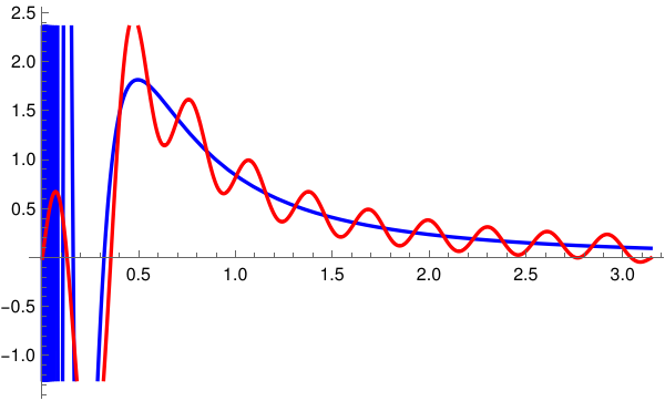
We can expand this function into sine-Fourier series \[ \frac{1}{x}\,\sin \left( \frac{1}{x} \right) = \sum_{n\ge 1} b_n \sin (nx) . \] With Mathematica, we can evaluate several coefficients, numerically. The following figure presents graph of function f(x) in blue, and its 20-term sine0Fourier approximation, in red.

   ■

Example 2: Let us define on (−π, π) the function \[ f(x) = \begin{cases} \frac{\sin (1/x)}{x\,\ln (1/|x|)} , &\quad 0 < |x| < e^{-2} , \\ 0, &\quad e^{-2} \le |x| \le \pi . \end{cases} \] This function is extended in odd way so its Fourier series will contain only sine functions. As usual, f is assumed to be 2π periodic because we extend it into the Fourier series.

The given function is not absolutely integrable because near zero, \[ |f(x)| \,\sim \, \frac{1}{|x|\,\ln (1/|x|)} . \] So \[ \int_0^{1/e^2} |f(x)|\,{\text d}x \ge \int_0^{1/e^2} \frac{{\text d}x}{|x|\,\ln (1/|x|)} . \] Substitude t = ln(1/x), then dx = −e^−tdt, and we get \[ \int_0^{1/e^2} |f(x)|\,{\text d}x \ge \int_2^{+\infty} \frac{{\text d}t}{t} = \infty . \] So f ∉ 𝔏¹([−π, π). However, the Fourier sine coefficients exist: \[ b_n = \frac{2}{\pi} \int_0^{\pi} f(x)\,\sin (nx)\,{\text d}x = \frac{2}{\pi} \int_0^{1/e^2} \,\frac{\sin (1/x)}{x\,\ln (1/x)}\,\sin (nx)\,{\text d}x . \] Let t = 1/x, then dx = −dt/t² and ln(1/x) = ln(t). Then \[ b_n = \frac{2}{\pi} \int_{e^2}^{\infty} \frac{\sin t}{\left( 1/t \right) \ln t}\,\sin \left( \frac{n}{t} \right) \frac{{\text d}t}{t^2} = \frac{2}{\pi} \int_{e^2}^{\infty} \frac{\sin t\,\sin (n/t)}{t\,\ln t} \,{\text d}t . \] For large t, \[ \sin \left( \frac{n}{t} \right) \,\sim \,\frac{n}{t} , \] so the integrand behaves like \[ \frac{\sin t}{t\,\ln t} \cdot \frac{n}{t} = n\,\frac{\sin t}{t^2 \ln t} . \] Now \[ \int_{e^2}^{\infty} \left\vert \frac{\sin t}{t^2 \ln t} \right\vert {\text d}t \le \int_{e^2}^{\infty} \frac{{\text d}t}{t^2 \ln t} < \infty . \] Hence, the integral defining bₙ converges absolutely for each n. Thus, all Fourier coefficients exist, even so f ∉ 𝔏¹.

However, the corresponding Fourier series converges very slow because bₙ ∼ 1/lnn (see section).    ■

Example 3:    ■