Return to computing page for the first course APMA0330computing page for the second course APMA0340computing page for the fourth course APMA0360Mathematica tutorial for the first course APMA0330Mathematica tutorial for the second course APMA0340Mathematica tutorial for the fourth course APMA0360main page for the first course APMA0330main page for the second course APMA0340main page for the fourth course APMA0360Part V of the course APMA0340 Linear Algebra with Mathematica
This section is a collection of Fourier series expansions for different
functions.
Theorem: If a periodic function of period \( 2\ell \) is
square-integrable on any finite interval, then the Fourier series converges to the function at almost every point:
\[
f(x) \,\sim \, \frac{a_0}{2} + \sum_{k\ge 0} \left[ a_k \cos \left( \frac{k \pi x}{\ell} \right) + b_k \sin \left( \frac{k \pi x}{\ell} \right) \right] ,
\]
where its coefficients are determined via Euler--Fourier formula:
\[
\begin{split} a_k &= \frac{1}{\ell} \, \int_{-\ell}^{\ell} f(x)\,\cos \left( \frac{k \pi x}{\ell} \right) {\text d} x , \quad k=0,1,2,\ldots ,
\\
b_k &= \frac{1}{\ell} \, \int_{-\ell}^{\ell} f(x)\,\sin \left( \frac{k \pi x}{\ell} \right) {\text d} x , \quad k=1,2,\ldots .
\end{split} \qquad\qquad ■
\]
Expansion in a
complex form (or exponential form):
\begin{equation} \label{EqFourier.1}
f(x) \,\sim\, \mbox{P.V.}\sum_{n=-\infty}^{\infty} \hat{f}(n)\, e^{n{\bf j} \pi x/\ell} = \lim_{N\to \infty} \sum_{n=-N}^{N} \hat{f}(n)\, e^{n{\bf j} \pi x/\ell} ,
\end{equation}
where
T = 2ℓ is the period and the Fourier coefficients
\( \hat{f}(n) \) are evaluated according to the Euler--Fourier formula:
\begin{equation} \label{EqFourier.2}
\hat{f}(n) = \frac{1}{2\ell} \int_{-\ell}^{\ell} f(x)\, e^{-n{\bf j} \pi x/\ell} \,{\text d} x = \frac{1}{T} \int_{0}^{T} f(x)\, e^{-2n{\bf j} \pi x/T} \,{\text d} x , \qquad n \in \mathbb{Z} = \left\{ 0, \pm 1, \pm 2, \ldots \right\} .
\end{equation}
Here «P.V.» abbreviates the
Cauchy principle value , which is a regularization of the infinite sum.
The first examples are based on well-known sum of geometric series
\[
\frac{1}{2} + z + z^2 + z^3 + \cdots = \frac{1}{2} \cdot \frac{1+z}{1-z} ,
\]
where
\( z = r\,e^{{\bf j}x} . \) Extraction of real and imaginary parts yields the following series:
\[
P(r, x) = \frac{1}{2} + \sum_{n\ge 1} r^n \cos (nx) = \mbox{P.V.} \sum_{n = -\infty}^{\infty} r^{|n|} e^{{\bf j}nx} = \frac{1}{2} \cdot \frac{1 + r^2}{1- 2r\,\cos x + r^2} ,
\]
\[
Q(r, x) =\sum_{n\ge 1} r^n \sin (nx) = \frac{1}{2} \cdot \frac{r\, \sin x}{1- 2r\,\cos x + r^2} .
\]
The function
P (
r, x ) is called the
Poisson kernel .
Similarly, from the formula
\[
\ln \frac{1}{1-z} = z + \frac{1}{2}\, z^2 + \frac{1}{3}\, z^3 + \frac{1}{4}\, z^4 + \cdots \qquad (0 \le r < 1),
\]
we get
\[
\sum_{n\ge 1} \frac{\cos nx}{n}\,r^n = \frac{1}{2} \cdot \ln \frac{1}{1 - 2r\,\cos x + r^2} , \qquad \sum_{n\ge 1} \frac{\sin nx}{n}\, r^n = \arctan \frac{r\,\sin x}{1 - 2r\,\cos x + r^2} .
\]
From these sums, we derive
\begin{eqnarray*}
\sum_{n\ge 1} \frac{1}{n} \, \cos n x &=& -\frac{1}{2} \, \ln \left[ 2 \left( 1 - \cos x \right) \right] , \qquad \mbox{on interval } \ 0 < x < 2\pi ;
\\
\sum_{n\ge 1} \frac{1}{n} \, \sin n x &=& \begin{cases}
\phantom{-}\frac{\pi -x}{2} , & \ \mbox{for } 0< x < \pi , \\
- \frac{\pi +x}{2} , & \ \mbox{for } -\pi < x < 0 ,
\end{cases} \qquad \mbox{on interval } \ -\pi < x < \pi .
\\
\sum_{n\ge 1} \frac{1}{n} \, \sin \frac{n\pi x}{\ell} &=& \frac{\ell-x}{2}
, \qquad 0 < x < 2\ell .
\\
\sum_{n\ge 1} \frac{(-1)^{n+1}}{n} \, \cos n x &=& \ln \left( 2 \, \cos \frac{x}{2} \right) , \qquad \mbox{on interval } \ |x| < \pi ;
\\
\sum_{n\ge 1} \frac{(-1)^{n+1}}{n} \, \sin n x &=& \frac{x}{2} , \qquad \mbox{on interval } \ |x| < \pi .
\end{eqnarray*}
\[
\frac{1}{2{\bf j}}\,\sum_{n\ne 0} \frac{e^{{\bf j}nx}}{n} = \begin{cases}
- \frac{\pi}{2} - \frac{x}{2} , & \ \mbox{ if} \quad -\pi < x < 0 ,
\\ 0 , & \ \mbox{ if} \quad x = 0,
\\
\frac{\pi}{2} - \frac{x}{2} , & \ \mbox{ if} \quad 0 < x < \pi .
\end{cases}
\]
S1[x_] = Sum[1/n*Cos[n*x] , {n, 1, 100}];
S2[x_] = Sum[1/n*Sin[n*x], {n, 1, 100}];
S3[x_] = Sum[1/n*Sin[(n*\[Pi]*x)/l], {n, 1, 100}];
S4[x_] = Sum[(-1)^(n + 1)/n*Cos[n*x], {n, 1, 100}];
S6[x_] = 1/(2 \[ImaginaryJ]) Sum[E^(\[ImaginaryJ]*n*x)/n, {n, 1, 100}];
\begin{eqnarray*}
\sum_{n\ge 1} \frac{1}{2n-1} \, \cos (2n-1) x &=& \frac{1}{2} \cdot \ln \left( \cot \frac{x}{2} \right) ,
\qquad \mbox{on interval } \ 0 < x < \pi .
\\
\sum_{n\ge 1} \frac{1}{2n-1} \, \sin (2n-1) x &=& \frac{1}{2} \sum_{\nu =-\infty}^{+\infty} \frac{e^{{\bf j}\left( 2\nu -1 \right) x}}{{\bf j} \left( 2\nu -1 \right)} = \frac{\pi}{4} \cdot \mbox{sign} (x) = \frac{\pi}{4} \times \begin{cases}
\phantom{-}1 , & \ \mbox{for } 0< x , \\
- 1 , & \ \mbox{for } x<0 ,
\end{cases} \qquad \mbox{on interval } \ -\pi < x < \pi .
\\
\frac{4}{\pi}\,\sum_{n\ge 1} \frac{1}{2n-1} \, \sin \frac{(2n-1)\pi x}{\ell} &=& 2 \left[ H\left( \frac{x}{\ell} \right) - H\left( \frac{x}{\ell} -1 \right) \right] -1 .
\\
\sum_{n\ge 1} \frac{(-1)^{n+1}}{2n-1} \, \cos (2n-1) x &=&
\begin{cases}
\phantom{-}\frac{\pi}{4} , & \ \mbox{for } 0 < x < \frac{\pi}{2} , \\
-\frac{\pi}{4} , & \ \mbox{for } -\frac{\pi}{2} < x < 0 ,
\end{cases} \qquad \mbox{on interval } \ -\frac{\pi}{2} < x < \frac{\pi}{2} .
\\
\sum_{n\ge 1} \frac{(-1)^{n+1}}{2n-1} \, \sin (2n-1) x &=& \frac{1}{2} \,\ln \left\vert \cot \left( \frac{x}{2} - \frac{\pi}{4} \right) \right\vert , \qquad \mbox{everywhere} ,
\end{eqnarray*}
where
H is the Heaviside function.
S7[x_] = Sum[1/(2*n - 1)*Cos[(2*n - 1)*x], {n, 1, 100}];
S8[x_] = Sum[1/(2*n - 1)*Sin[(2*n - 1)*x], {n, 1, 100}];
Manipulate[
Plot[{4/\[Pi]*Sum[Sin[((2 n - 1)*\[Pi]*t)/l]/(2*n - 1), {n, 1, 100}],
2*(HeavisideTheta[t/l] - HeavisideTheta[t/l - 1]) - 1}, {t, -10,
10}, PlotStyle -> {{Thickness[0.01], Orange}, {Thickness[0.01],
Blue}}], {l, 1, 5}]
S10[x_] = Sum[(-1)^(n + 1)/(2 n - 1)*Cos[(2 n - 1)*x], {n, 1, 100}];
S11[x_] = Sum[(-1)^(n + 1)/(2 n - 1)*Sin[(2 n - 1)*x], {n, 1, 100}];
\begin{eqnarray*}
\frac{1}{2} + \sum_{n\ge 0} \frac{(-1)^n}{1+n^2} \left( \cos nx -n\,\sin nx \right) &=& \frac{\pi}{2\,\sinh \pi}\, e^x , \qquad \mbox{on interval } \ |x|< \pi .
\\
\frac{2}{\pi} - \frac{4}{\pi} \,\sum_{n\ge 1} \frac{1}{4n^2 -1} \, \cos 2nx &=& \sin x , \qquad \mbox{on interval } \ 0\le x < \pi .
\end{eqnarray*}
S12[x_] =
0.5 + Sum[(-1)^n/(1 + n^2)*(Cos[n*x] - n*Sin[n*x]), {n, 1, 100}];
S13[x_] = 2/\[Pi] - 4/\[Pi]*Sum[1/(4*n^2 - 1)*Cos[2*n*x], {n, 1, 100}];
\begin{eqnarray*}
\sum_{n\ge 1} \frac{(-1)^{n+1}}{n^2} \, \cos n x &=& - \frac{x^2}{4} + \frac{\pi^2}{12} , \qquad \mbox{on interval } \ |x| < \pi .
\\
\sum_{n\ge 1} \frac{(-1)^{n+1}}{n^2} \, \sin n x &=& -\mbox{Cl}_2 (\pi +x) = -\mbox{Cl}_2 (x- \pi ) = \int_0^{\pi +x} \, \ln \left\vert 2\,\sin \left( \frac{x}{2} \right) \right\vert {\text d}x, \qquad \ |x| < \pi ,
\\
\sum_{n\ge 1} \frac{1}{n^2} \, \cos n x &=& \frac{(x-\pi )^2}{4} - \frac{\pi^2}{12}, \qquad \mbox{on interval } \ 0< x < 2\pi .
\\
\sum_{n\ge 1} \frac{\sin n x}{n^2} \, \sin n x &=& \mbox{Cl}_2 (x) = -\int_0^{x} \, \ln \left\vert 2\,\sin \left( \frac{x}{2} \right) \right\vert {\text d}x = \Im \left( \mbox{Li}_2 \left( e^{\mathbf{j}\,x} \right) \right) , \qquad \ 0 < x < 2\pi .
\end{eqnarray*}
where Cl₂(
y ) is the
Clausen function of order 2, and Li₂ is the
dilogarithm (or Spence's function):
\( \displaystyle \quad \mbox{Li}_2 (z) = \sum_{m\ge 1} \,\frac{z^m}{m^2} =- \int_0^z \,\frac{\ln (1-u)}{u}\,{\text d}u , \quad z \in \mathbb{C} , \quad \)
There is no restriction such as ∣
x ∣ < π for the Fourier series itself. That interval is sometimes chosen merely as a fundamental domain because Cl₂ is an odd, 2π-periodic function. In general,
\[
\mbox{Li}_2 \left( e^{\mathbf{j}\vartheta} \right) = \mbox{GL}_2 (\vartheta ) + \mathbf{j}\,\mbox{Cl}_2 (\vartheta ) = \sum_{k\ge 1}\,\frac{\cos (k\vartheta )}{k^2} + \mathbf{j}\,\sum_{k\ge 1}\,\frac{\sin (k\vartheta )}{k^2}
\]
Sum[Cos[n*x]/n^2 , {n, 1, Infinity}]
1/2 (PolyLog[2, E^(-I x)] + PolyLog[2, E^(I x)])
S14[x_] = Sum[(-1)^(n + 1)/n^2*Cos[n*x], {n, 1, 100}];
S15[x_] = Sum[(-1)^(n + 1)/n^2*Sin[n*x], {n, 1, 100}];
S16[x_] = Pi^2/12 + Sum[Cos[n*x]/n^2, {n, 1, 20}] ;
S17[x_] = Sum[1/n^2*Sin[x], {n, 1, 100}];
\begin{eqnarray*}
\sum_{n\ge 1} \,\frac{1}{(2n-1)^2} \ \cos (2n-1) x &=& G + \frac{\pi^2}{8} - \frac{\pi |x|}{4} , \qquad \mbox{on interval } \ |x| < \pi ;
\\
\sum_{n\ge 1} \frac{1}{(2n-1)^2} \ \sin (2n-1) x &=& \frac{1}{2}\,\mbox{Cl}_2 (x) - \frac{1}{2}\, \mbox{Cl}_2 (\pi -x) = \frac{1}{2}\,\int_0^x \,\ln \left( \cot \frac{t}{2} \right) {\text d}t , \qquad \mbox{on interval } \ 0 \le x \le \pi .
\\
\sum_{n\ge 1} \,\frac{(-1)^{n+1}}{(2n-1)^2} \ \cos (2n-1) x &=& K + \frac{1}{2}\,\mbox{Cl}_2 (\pi - 2|x|) , \qquad \mbox{on interval } \ |x| < \pi ;
\\
\sum_{n\ge 1} \,\frac{(-1)^{n+1}}{(2n-1)^2} \ \sin (2n-1) x &=& \frac{\pi x}{4} ,
% \int_0^x \,\ln \left\vert \cot \frac{t}{2} \right\vert {\text d}t = \frac{1}{2} \left( \mbox{Cl}_2 (x) + \mbox{Cl}_2 (\pi -x) \right) = \frac{1}{2}\,\Im \left\{ \mbox{Li}_2 \left( -\mathbf{j}\,e^{\mathbf{j}\,x} \right) - \mbox{Li}_2 \left( \mathbf{j}\,e^{\mathbf{j}\,x} \right) \right\} ,
\qquad \mbox{on interval } \ -\frac{\pi}{2} \le x \le \frac{\pi}{2} .
\end{eqnarray*}
where
\( \displaystyle \quad K = \sum_{k\ge 0} \frac{(-1)^k}{(2k+1)} \,\approx; 0.915965 \ \) is
Catalan's constant and the
Clausen function :
\( \displaystyle \quad \mbox{Cl}_2 (\theta ) = -\int_0^{\theta} \,\ln \left( 2\,\sin \frac{t}{2} \right) {\text d}t . \)
f[x_] := Sum[Sin[(2 n - 1) x]/(2 n - 1)^2, {n, 1, Infinity}]
-(1/8) I E^(-I x) (-LerchPhi[E^(-2 I x), 2, 1/2] +
E^(2 I x) LerchPhi[E^(2 I x), 2, 1/2])
g[x_] := ClausenCl[2, x] - 1/4 ClausenCl[2, 2 x]
h[x_] := (ClausenCl[2, x] + ClausenCl[2, Pi - x])/2
FullSimplify[g[x] == h[x], 0 <= x <= Pi]
Plot[
Evaluate[{f[x], g[x]}],
{x, 0, Pi},
PlotLegends -> {"Fourier series", "Closed form"}
]
S18[x_] = Sum[Cos[(2*n - 1)*x]/(2*n - 1)^2, {n, 1, 100}];
S19[x_] = Sum[Sin[(2 n - 1)*x]/(2 n - 1)^2, {n, 1, 100}];
\[
\begin{split}
\sum_{n\ge 1} \,\frac{1}{n^3} \, \cos n x &= \zeta (3) + \int_0^x \,\left( x - u \right) \ln \left( 2\,\sin \frac{u}{2} \right) {\text d}u = \Re \left( \mbox{Li}_3 \left( e^{\mathbf{j}\,x} \right) \right)
, \qquad
\\
\sum_{n\ge 1} \,\frac{(-1)^n}{n^3} \, \cos n x &= \mbox{Cl}_3 (x+ \pi ) = \Re \left( \mbox{Li}_3 \left( - e^{\mathbf{j}\,x} \right) \right) , \qquad
\\
\sum_{n\ge 1} \frac{1}{n^3} \, \sin n x &= \frac{\pi^2 x}{6} - \frac{\pi x^2}{4} + \frac{x^3}{12} , \qquad \mbox{on interval } \ 0 < x < 2\pi .
\\
\sum_{n\ge 1} \frac{(-1)^n}{n^3} \, \sin n x &= \frac{x^3 - \pi^2 x}{12} \qquad \mbox{on interval } \ |x| \le \pi .
\\
\sum_{n\ge 1} \frac{1}{n^3} \, \sin (2n x) &= \frac{1}{6} \times \begin{cases}
4 x^3 + 6\pi x^2 + 2 \pi^2 x , & \quad\mbox{for} \quad x \in (-\pi ,0) ,
\\
4 x^3 - 6\pi x^2 + 2 \pi^2 x , & \quad\mbox{for} \quad x \in (0, \pi) .
\end{cases}
\\
\sum_{n\ge 1} \frac{e^{\mathbf{j}\,nx}}{n^3} &= \mbox{Li}_3 \left( e^{\mathbf{j}\,x} \right) ,
\end{split}
\]
where Li₃(
x ) is the
trilogarithm . Note that
\( \displaystyle \quad \mbox{Cl}_3 (x) = \Re \left( \mbox{li}_3 \left( e^{\mathbf{j}\,x} \right) \right) . \)
Sum[Cos[n*x]/n^3, {n, 1, Infinity}]
1/2 (PolyLog[3, E^(-I x)] + PolyLog[3, E^(I x)])
Some famous sums:
\begin{align*}
\sum_{n\ge 1} \,\frac{\cos (n\theta )}{n^{4}} &= \frac{\pi^4}{90} - \frac{\theta^2 \pi^2}{12} + \frac{\theta^3 \pi}{12} - \frac{\theta^4}{48} , \qquad 0 \le x \le 2\pi ,
\\
\sum_{n\ge 1} \,\frac{\sin (n\theta )}{n^{5}} &= \frac{\theta\,\pi^4}{90} - \frac{\theta^3 \pi^2}{36} + \frac{\theta^4 \pi}{48} - \frac{\theta^5}{240} , \qquad 0 \le x \le 2\pi .
\end{align*}
s30[x_] = Sum[Cos[n*x]/n^4, {n, 1, 30}];
f4[x_] = Pi^4 /90 - Pi^2 * x^2 /12 + Pi*x^3 /12 - x^4 /48;
Plot[{f4[x], s30[x]}, {x, -2, 8}, PlotStyle -> Thick]
s25[x_] = Sum[Sin[n*x]/n^5, {n, 1, 25}];
f[x_] = Pi^4 *x/90 - Pi^2 * x^3 /36 + Pi*x^4 /48 - x^5 /240;
Plot[{f[x], s25[x]}, {x, -2, 8}, PlotStyle -> Thick]
In general,
\[
\sum_{n\ge 1} \,\frac{\sin (n\theta )}{n^{2m}} = \mbox{Cl}_{2m} (\theta ) ,
\qquad
\sum_{n\ge 1} \,\frac{\cos (n\theta )}{n^{2m+1}} = \mbox{Gl}_{2m+1} (\theta ) ,
\]
s20[x_] := Sum[(-1)^n Cos[n x]/n^3, {n, 1, 20}];
f[x_] := Re[PolyLog[3, -Exp[I x]]];
Plot[Evaluate[{f[x], s20[x]}], {x, -Pi, Pi},
PlotStyle -> {{Red, Thick}, {Blue, Thick}},
PlotLegends -> {"Exact", "20 terms", "Error"}, PlotRange -> All]
S21[x_] = Sum[Cos[n*x]/n^3, {n, 1, 100}];
S22[x_] = Sum[(-1)^n *Cos[n*x]/n^3, {n, 1, 100}];
S23[x_] = Sum[Sin[n*x]/n^3, {n, 1, 100}];
S23a[x_] = Sum[Sin[2*n*x]/n^3, {n, 1, 100}];
S24[x_] = Sum[(-1)^n *Sin[n*x]/n^3, {n, 1, 100}];
\[
\frac{8}{\pi} \,\sum_{n\ge 1} \frac{1}{(2n-1)^3}\ \sin\left( 2n-1 \right) x =
\pi x - |x|\,x
= \begin{cases}
x \left( \pi - x \right) , & \quad 0 \le x \le \pi ,
\\
-x \left( \pi + x \right) , & \quad -\pi \le x \le 0.
\end{cases}
\]
S25[x_] = 8/\[Pi]*Sum[Sin[(2 n - 1)*x]/(2 n - 1)^3, {n, 1, 100}];
p251 = Plot[S25[t], {t, -\[Pi], \[Pi]},
PlotStyle -> {Thickness[0.02], Orange}];
f[x_] = Piecewise[{{x*(Pi-x), 0
p252 = Plot [f[t], {t, -\[Pi], Pi},
PlotStyle -> {Thickness[0.007], Blue}];
Show[p251, p252]
\[
\sum_{n\ge 1} \frac{1}{(2n-1)^3}\,\cos\left( 2n-1 \right) x = \frac{7}{8}\,\zeta (3) + \frac{1}{2} \,\int_0^x \left( \mbox{Cl}_2 (t) + \mbox{Cl}_2 (\pi -t ) \right) {\text d}t ,
\]
where
\( \displaystyle \quad \zeta(3) = \sum_{n\ge 1} \,\frac{1}{n^3} \, \approx 1.2020569\ldots \quad \) is
Apéry's constant .
S26[x_] = Sum[Cos[(2 n - 1)*x]/(2 n - 1)^3, {n, 1, 100}];
\[
\begin{split}
\sum_{n\ge 1} \,\frac{(-1)^n}{(2n-1)^3}\ \sin\left( 2n-1 \right) x &=
\left[ \mbox{Cl}_3 (x - \pi /2) - \frac{1}{8}\,\mbox{Cl}_3 (2x-\pi ) - \mbox{Cl}_3 (x + \pi /2) + \frac{1}{8}\,\mbox{Cl}_3 (2x+\pi ) \right]
\\
&=
\frac{1}{2}\,\Re \left[ \mbox{Li}_3 \left( e^{\mathbf{j} \left( x + \pi /2\right)} \right) - \mbox{Li}_3 \left( e^{\mathbf{j} \left( x - \pi /2\right)} \right) \right] ,
\qquad \mbox{on interval } \ -\frac{\pi}{2} \le x < < 2\pi ;
\\
\sum_{n\ge 1} \frac{(-1)^n}{(2n-1)^3}\,\cos\left( 2n-1 \right) x &= -\mbox{Cl} (x+\pi ) + \frac{1}{8}\,\mbox{Cl}_3 (2x) = \Im\,\mbox{Li}_3 \left( -e^{\mathbf{j}\,x} \right) + \frac{1}{8}\,\Re\,\mbox{Li}_3 \left( -e^{2\mathbf{j}\,x} \right) , , \qquad \mbox{on interval } \ 0< x < < 2\pi ;
\end{split}
\]
s30[x_] = Sum[(-1)^n * Sin[(2*n - 1)*x]/(2*n - 1)^3 , {n, 1, 30}];
f[x_] :=
1/2 Re[PolyLog[3, Exp[I (x + Pi/2)]] -
PolyLog[3, Exp[I (x - Pi/2)]]];
g[x_] := Sum[(-1)^n Sin[(2 n - 1) x]/(2 n - 1)^3, {n, 1, Infinity}];
Plot[{s30[x], f[x]}, {x, -Pi/2, Pi*2}]
S27[x_] = Sum[(-1)^n/(2*n - 1)^3*Sin[(2*n - 1)*x], {n, 1, 100}];
\begin{align*}
\sum_{n\ge 1} \,\frac{(-1)^{n-1}}{n^4}\ \cos\left( n\,x \right) &= \frac{x^4}{48} - \frac{\pi^2}{24}\, x^2 + \frac{7 \pi^4}{720} , \qquad |x| < \pi .
\\
\sum_{n\ge 1} \,\frac{1}{n^4}\ \cos\left( n\,x \right) &= \frac{\pi^4}{90} - \frac{\pi^2}{12}\,x^2 + \frac{\pi}{12}\,x^3 - \frac{x^4}{48}, \qquad 0 \le y \le 2\pi ,
\\
\sum_{n\ge 1} \,\frac{(-1)^{n-1}}{n^4}\ \sin\left( n\,x \right) &= \mbox{Cl}_4 (x+\pi ) = -\Im\,\mbox{Li}_4 \left( - e^{\mathbf{j}\,x} \right) , \qquad |x| < \pi .
\\
\sum_{n\ge 1} \,\frac{1}{n^4}\ \sin\left( n\,x \right) &= \mbox{Cl}_4 (x) = \Im\left( \mbox{Li}_4 \left( e^{\mathbf{j}\,x} \right) \right), \qquad 0 \le y \le 2\pi .
\end{align*}
S[x_] = -48*Sum[(-1)^n *Cos[n*x]/n^4, {n, 1, 100}];
The general rule:
\[
\sum_{n\ge 1} \frac{\cos (nx)}{n^{2m}} \quad\mbox{and} \quad \sum_{n\ge 1} \frac{\sin (nx)}{n^{2m+1}} \quad\mbox{are piecewise Bernoulli polynomials} ,
\]
\[
\sum_{n\ge 1} \frac{\cos (nx)}{n^{2m+1}} \quad\mbox{and} \quad \sum_{n\ge 1} \frac{\sin (nx)}{n^{2m}} \quad\mbox{are generalized Clausen (polylogarithmic)} .
\]
✔ ✘
Series
Closed form (0 ≤ x ≤ 2π)
Bernoulli connection
\(\displaystyle \quad\sum_{n\ge1}\frac{\sin(nx)}{n} \qquad \)
\(\displaystyle \quad \frac{\pi-x}{2}\)
\(\displaystyle\quad -\pi\,B_1\!\left(\frac{x}{2\pi}\right)\)
\(\displaystyle \quad\sum_{n\ge1}\frac{\cos(nx)}{n^2} \qquad \)
\(\displaystyle \quad \frac{\pi^2}{6}-\frac{\pi x}{2}+\frac{x^2}{4}\)
\(\displaystyle \quad \pi^2\,B_2\!\left(\frac{x}{2\pi}\right)\)
\(\displaystyle\quad \sum_{n\ge1}\frac{\sin(nx)}{n^2}\)
\( \quad \operatorname{Cl}_2(x)\)
First genuinely non-elementary case
\(\displaystyle \quad\sum_{n\ge1}\frac{\cos(nx)}{n^3}\)
\(\displaystyle \quad \zeta(3)-\int_0^x\operatorname{Cl}_2(t)\,{\text d}t\)
Integral of a Clausen function
\(\displaystyle \quad \sum_{n\ge1}\frac{\sin(nx)}{n^3}\)
\(\displaystyle \quad \frac{\pi^2x}{6}-\frac{\pi x^2}{4}+\frac{x^3}{12}\)
\(\displaystyle \quad\frac{2\pi^3}{3}\,B_3\!\left(\frac{x}{2\pi}\right)\)
\(\displaystyle \quad \sum_{n\ge1}\frac{\cos(nx)}{n^4}\)
Quartic polynomial
\(\displaystyle \quad -\frac{\pi^4}{3}\,B_4\!\left(\frac{x}{2\pi}\right)\)
First few Bernoulli polynomials:
\begin{align*}
B_1 (t) &= t - \frac{1}{2} , \\
B_2 (t) &= t^2 -t + \frac{1}{6} , \\
B_3 (t) &= t^3 - \frac{3}{2}\, t^2 + \frac{1}{2}\,t , \\
B_4 (t) &= t^4 - 2\,t^3 + t^2 - \frac{1}{30} .
\end{align*}
In fact, there is a beautiful theorem lurking behind these examples:
\[
\sum_{n\ge 1}\,\frac{\cos (nx)}{n^{2m}} = (-1)^{m+1}\,\frac{(2\pi )^{2m}}{2\left( 2m \right) !}\,B_{2m} \left( \frac{x}{2\pi} \right) ,
\]
and
\[
\sum_{n\ge 1}\,\frac{\sin (nx)}{n^{2m+1}} = (-1)^{m+1}\,\frac{(2\pi )^{2m+1}}{2\left( 2m+1 \right) !}\,B_{2m+1} \left( \frac{x}{2\pi} \right) ,
\]
valid on 0≤x≤2π (with periodic extension). These identities explain all of the elementary entries in the table at once, while the complementary parity naturally leads to the Clausen functions. This provides a very elegant bridge from Fourier series to Bernoulli polynomials and then to polylogarithms. See M. Abramowitz and I. A. Stegun (eds.), Handbook of Mathematical Functions, Chapter 23, §§23.1–23.2.
We will use the follwoing identities:
\[
(-\mathbf{j})^{2k+1} = (-1)^{k+1} \mathbf{j} , \qquad \cos (n\pi ) = (-1)^n , \quad 1 - \cos (n\pi ) = \begin{cases}
2, &\qquad \mbox{for } \ n = 2k+1 , \\
0, &\qquad \mbox{for } \ n = 2k .
\end{cases}
, \qquad n\\in \mathbb{Z} ,
\]
and
\[
\cos \left( n\,\frac{\pi}{2} \right) = \begin{cases}
0, \qquad& \mbox{for $n$ odd} , \\
(-1)^{n/2} , \qquad& \mbox{for $n$ even} ,
\end{cases} \qquad\quad
\sin \left( n\,\frac{\pi}{2} \right) = \begin{cases}
0, \qquad& \mbox{for $n$ even} , \\
(-1)^{(n-1)/2} , \qquad& \mbox{for $n$ odd} .
\end{cases}
\]
Example 1: square wave functions
Example 1: \( (0, 2\ell ) : \)
\begin{align*}
f(x) &= 2 \left[ H(x/\ell ) - H(x/\ell -1) \right] -1 = \begin{cases}
\phantom{-}1, & \ 0< x< \ell , \\ -1, & \ \ell < x < 2\ell ; \end{cases}
\\
g(x) &= H(x/\ell ) - H(x/\ell -1) = \begin{cases}
1, & \ 0< x< \ell , \\ 0, & \ \ell < x < 2\ell ; \end{cases}
\\
h(x) &= H(x/\ell -1) - H(x/\ell -2) = \begin{cases}
0, & \ 0< x< \ell , \\ 1, & \ \ell < x< 2\ell ; \end{cases}
\end{align*}
where
H(t) is the
Heaviside function . Since the function
g is
an odd function, all coefficients
a k are zeroes and we get
sine Fourier series (setting
\( \ell =1 \) for
simplicity):
\[
b_k = \int_0^2 f(x) \,\sin \left( k\pi x \right) {\text d}x = - \frac{4}{k\pi}
\,(-1)^k \sin^2 \frac{k\pi}{2} = \frac{4}{k\pi} \times \begin{cases}
1 , & \ \mbox{if $k$ is odd}, \\ 0, & \ \mbox{if $k$ is even}. \end{cases}.
\]
Therefore, we get the following Fourier series for
f(x) :
\[
f(x) = \frac{4\,\ell}{\pi}\, \sum_{n\ge 0} \,\frac{1}{2n+1} \, \sin \left(
\frac{(2n+1)\pi x}{\ell} \right) .
\]
Using
Mathematica ,
g[x_,L_]=HeavisideTheta[x/L] - HeavisideTheta[-1 + x/L]
we find other Fourier series:
\begin{align*}
g(x) &= \frac{\ell}{2} + \frac{2\ell}{\pi} \sum_{n\ge 0} \frac{1}{2n+1}\,
\sin \frac{(2n+1)\,\pi x}{\ell} ,
\\
h(x) &= \frac{\ell}{2} - \frac{2\ell}{\pi} \sum_{n\ge 0} \frac{1}{2n+1}\,
\sin \frac{(2n+1)\,\pi x}{\ell} .
\end{align*}
Then we plot partial sums with 10 terms (for simplicity setting
\( \ell =1 \) ):
ff[x_] = Sum[4/Pi/(2*n + 1)*Sin[(2*n + 1)*Pi*x], {n, 0, 10}]
The Fourier series for the characteristic function is
\[
\frac{b-a}{\ell} + \sum_{n\ge 1} \frac{1}{n\pi} \left( \sin \frac{n\pi b}{\ell} - \sin \frac{n\pi a}{\ell} \right) \cos \frac{n\pi x}{\ell} + \sum_{n\ge 1} \frac{1}{n\pi} \left( \cos \frac{n\pi a}{\ell} - \cos \frac{n\pi b}{\ell} \right) \sin \frac{n\pi x}{\ell} = \chi_{[a,b]} = \begin{cases}
1, & \ \mbox{ for }\ x \in [a,b] ,
\\
0, & \ \mbox{ otherwise.}
\end{cases}
\]
■
End of Example 1
Example 2: saw-tooth functions
Example 2:
\[
|x| = \begin{cases}
\phantom{-}x, & \ \mbox{ for} \quad 0 < x < \ell ,
\\
-x, & \ \mbox{ for} \quad -\ell < x 0; \ell
\end{cases}
\]
\[
f(x) = \begin{cases}
\frac{\ell - x}{2} , & \ \mbox{ for } \ 0 < x < \ell ,
\\
\frac{\ell + x}{2} , & \ \mbox{ for } \ -\ell < x < 0 .
\end{cases}
\]
and
\[
g(x) = \begin{cases}
1 - |x|/\delta , & \ \mbox{ if } \ |x| \le \delta ,
\\
0, & \ \mbox{ if } \ |x| > \delta .
\end{cases}
\]
Here δ is some small positive number. We expand these functions into Fourier series:
\begin{align*}
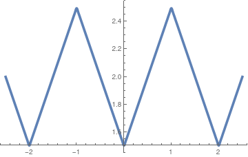
|x| &= 2 - \frac{4\ell}{\pi^2}\, \sum_{k\ge 1} \frac{1}{(2k-1)^2}\,\cos \frac{(2k-1)\pi x}{\ell} ,
\\
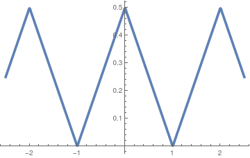
f(x) &= \frac{\ell}{4} - \frac{2\ell}{\pi^2} \, \sum_{k\ge 1} \frac{(-1)^k}{(2k-1)^2} \,\cos \frac{(2k-1) \pi x}{\ell}
\\
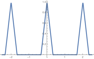
g(x) &= \frac{\delta}{2\ell} + \frac{2\ell}{\delta \pi^2} \,\sum_{n\ge 1} \frac{1}{n^2} \left[ 1 - \cos \frac{\delta n\pi}{\ell} \right] \cos \frac{n\pi x}{\ell} .
\end{align*}
Integrate[x*Cos[n*x*Pi/L], {x, 0, L}]*2/L
(2 L (-1 + Cos[n \[Pi]] + n \[Pi] Sin[n \[Pi]]))/(n^2 \[Pi]^2)
Integrate[(L - x)/2*Cos[n*x*Pi/L], {x, 0, L}]*2/L
(2 L Sin[(n \[Pi])/2]^2)/(n^2 \[Pi]^2)
Assuming[ d > 0,
Integrate[(1 - Abs[x]/d)*Cos[n*x*Pi/L], {x, 0, d}]*2/L]
(2 L (-1 + Cos[(d n \[Pi])/L]))/(d n^2 \[Pi]^2)
We plot these functions.
Fig.1: Graph of |x |
Fig.2: Graph of f (x )
Fig.3: Graph of g (x )
s20[x_] =
2 - (4/Pi^2)*Sum[Cos[Pi*(2*k - 1) *x]/(2*k - 1)^2 , {k, 1, 20}];
■
End of Example 2
Example 3: Heaviside function and its multiples
Example 3: n ℓ (n ∈ ℤ), where its is undefined. If you are familiar with generating functions, you should recognize that the derivative of the Heaviside function (in terms of distributions) is the Dirac delta function .
The Fourier series is pointwise convergent everywhere with the sum function H (t ):
\[
H(t) = \frac{1}{2} + \frac{2}{\pi} \ \sum_{k\ge 1}\, \frac{1}{2k-1}\ \sin \left( (2k-1)\,\frac{\pi}{\ell}\,t \right) ,
\]
because its coefficients are
\begin{align*}
a_0 &= \frac{1}{\ell} \,\int_0^{\ell}\, 1\,{\text d}t = 1 , \\
a_n &= \frac{1}{\ell} \,\int_0^{\ell}\, \cos \left( n\,\frac{\pi}{\ell}\,t \right) \,{\text d}t = 0, \\
b_n &= \frac{1}{\ell} \,\int_0^{\ell}\, \sin \left( n\,\frac{\pi}{\ell}\,t \right) \,{\text d}t = \frac{1 - \cos (n\pi )}{n\pi} , \qquad n=1,2,\ldots .
\end{align*}
a0 = Integrate[1, {x, 0, L}]/L
1
an = Integrate[Cos[n*Pi*x/L], {x, 0, L}]/L
Sin[n \[Pi]]/(n \[Pi])
bn = Integrate[Sin[n*Pi*x/L], {x, 0, L}]/L
(L - L Cos[n \[Pi]])/(L n \[Pi])
🔶 ❖ ♠ ♣
♥
♦ ❖ 🔶 ﹡ ⁎ ✱ ✲ ✳ ✺ ✻ ✼
✽ ❋
Example B: H (𝑡 − 𝑎), where 𝑎 ∈ (−ℓ, ℓ). Using Mathematica , we find the corresponding Fourier coefficients:
\begin{align*}
a_0 &= \frac{1}{\ell} \,\int_a^{\ell}\, 1\,{\text d}t = \frac{\ell - a}{\ell} , \\
a_n &= \frac{1}{\ell} \,\int_a^{\ell}\, \cos \left( n\,\frac{\pi}{\ell}\,t \right) \,{\text d}t = - \frac{1}{n\pi}\, \sin \left( \frac{an\pi}{\ell} \right), \\
b_n &= \frac{1}{\ell} \,\int_a^{\ell}\, \sin \left( n\,\frac{\pi}{\ell}\,t \right) \,{\text d}t = \frac{1}{n\pi} \left( \cos \left( \frac{an\pi}{\ell} \right) - (-1)^n \right) , \qquad n=1,2,\ldots .
\end{align*}
a0 = Integrate[Cos[0*Pi*x/L], {x, a, L}]/L
(-a + L)/L
an = Integrate[Cos[n*Pi*x/L], {x, a, L}]/L
(Sin[n \[Pi]] - Sin[(a n \[Pi])/L])/(n \[Pi])
bn = Integrate[Sin[n*Pi*x/L], {x, a, L}]/L
(-Cos[n \[Pi]] + Cos[(a n \[Pi])/L])/(n \[Pi])
Then the corresponding Fourier series becomes
\[
H(t-a) = \frac{\ell - a}{2\ell} = \sum_{n\ge 1} \,\frac{1}{n\pi} \left[ \left( \cos \left( \frac{an\pi}{\ell} \right) - (-1)^n \right) \cos \left( \frac{n\pi x}{\ell} \right) + \left( \cos \left( \frac{an\pi}{\ell} \right) - (-1)^n \right) \sin \left( \frac{n\pi x}{\ell} \right) \right] .
\]
🔶 ❖ ♠ ♣
♥
♦ ❖ 🔶 ﹡ ⁎ ✱ ✲ ✳ ✺ ✻ ✼
✽ ❋
,
Example C: f (𝑡) = H (𝑡)sin(𝑡). It is natural to consider this function on interval {−π, π] and the expand it periodically with period 2π. Then 𝑓(𝑡) will be continuous on whole line ℝ. Moreover, it is piecewise smooth ℭ¹, and its derivative has finite discontinuities at 𝑡 = n π (n ∈ ℤ) being corner points of the given function 𝑓(𝑡).
Since 𝑓(𝑡) is piecerwise smooth, it has convergent everywhere Fourier series, and its coefficients are evaluated by the standard Euler--Fourier formulas:
\begin{align*}
a_0 &= \frac{1}{\pi} \,\int_0^{\pi}\, \sin x\,{\text d}t = \frac{2}{\pi} , \\
a_n &= \frac{1}{\pi} \,\int_0^{\pi}\ \sin t\, \cos \left( n\,t \right) \,{\text d}t = \frac{1 + (-1)^n}{\left( 1 - n^2 \right) \pi} , \qquad n\ne 1, \\
b_n &= \frac{1}{\pi} \,\int_0^{\pi}\, \sin t\,\sin \left( n\,t \right) \,{\text d}t = \frac{1}{2}\,\delta_{n,1} , \qquad n=1,2,\ldots .
\end{align*}
a0 = Integrate[Sin[x], {x, 0, Pi}]/Pi
2/\[Pi]
an = Integrate[Sin[x]*Cos[n*x], {x, 0, Pi}]/Pi
(1 + Cos[n \[Pi]])/((1 - n^2) \[Pi])
bn = Integrate[Sin[x]*Sin[n*x], {x, 0, Pi}]/Pi
-(Sin[n \[Pi]]/((-1 + n^2) \[Pi]))
\[
H(t)\,\sin t = \frac{1}{\pi} + \frac{1}{2}\,\sin t + \frac{2}{\pi}\ \sum_{k\ge 1}\,\frac{1}{1 - 4 k^2}\ \cos \left( 2k\,x \right) .
\]
s20[x_] =
1/Pi + Sin[x]/2 + Sum[Cos[2*k*x]/(1 - 4*k^2), {k, 1, 20}]*(2/Pi);
Plot[{HeavisideTheta[x]*Sin[x], s20[x]}, {x, -Pi, 2*Pi},
PlotStyle -> Thick]
Since the first derivative of 𝑓(𝑡) is discontinuous, its Fourier coefficients decay as O*1/
n ²).
If we set 𝑡 = 0, we get
\[
0 = H(0)\,\sin (0) = \frac{1}{\pi} + \frac{2}{\pi}\ \sum_{k\ge 1}\,\frac{1}{1 - 4 k^2} .
\]
This leads to the identity:
\[
\sum_{k\ge 1}\,\frac{1}{4 k^2 -1} = \frac{1}{2} .
\]
🔶 ❖ ♠ ♣ ♥
♦ ❖ 🔶 ﹡ ⁎ ✱ ✲ ✳ ✺ ✻ ✼
✽ ❋
,
Example D: n ). Note that its derivative is zero almost everywhere. First, using Mathematica , we evaluate the Fourier coefficients:
\begin{align*}
a_0 &= \frac{1}{\pi} \,\int_{-\pi /2}^{\pi /2}\, \,{\text d}t = 0 , \\
a_n &= \frac{1}{\pi} \,\int_{-\pi /2}^{\pi}\ \cos \left( n\,t \right) \,{\text d}t = \frac{2}{n\pi} \cdot \sin \left( \frac{n\pi}{2} \right)n , \qquad n\ne 1, \\
b_n &= \frac{1}{\pi} \,\int_{-\pi /2}^{\pi}\,\,\sin \left( n\,t \right) \,{\text d}t = 0 , \qquad n=1,2,\ldots .
\end{align*}
an = Integrate[1*Cos[n*x], {x, -Pi/2, Pi/2}]/Pi
(2 Sin[(n \[Pi])/2])/(n \[Pi])
🔶 ❖ ♠ ♣
♥
♦ ❖ 🔶 ﹡ ⁎ ✱ ✲ ✳ ✺ ✻ ✼
✽ ❋
,
Example E:
bn = Integrate[Sin[x]*Sin[n*x], {x, -Pi/2, Pi/2}]/Pi
(2 n Cos[(n \[Pi])/2])/((-1 + n^2) \[Pi])
This yields the Fourier series
\[
f_5 (t) = \frac{1}{2}\,\sin t + \frac{4}{\pi}\,\sum_{k\ge 1} \ \frac{k}{4k^2 -1} \ \sin \left( 2kt \right) .
\]
■
End of Example 3
Example 4: Piecewise continuous functions
Example 4:
End of Example 4
\begin{align*}
x &= - \frac{2\ell}{\pi} \sum_{n\ge 1} \frac{(-1)^n}{n}\,\sin \left( \frac{n\pi x}{\ell} \right) , \qquad 0 < x < \ell ,
\\
&= - \frac{4\ell}{\pi^2} \sum_{k\ge 1} \frac{1}{(2k-1)^2}\,\cos \left( \frac{\left( 2k-1 \right) \pi x}{\ell} \right) , \qquad 0 < x < \ell .
\end{align*}
2*Integrate[x*Sin[Pi*n*x/L], {x, 0, L}]/L
(2 L (-n \[Pi] Cos[n \[Pi]] + Sin[n \[Pi]]))/(n^2 \[Pi]^2)
\begin{align*}
x^2 &= \frac{2\ell^2}{\pi^3} \sum_{n\ge 1} \frac{-2 +(-1)^n \left( 2- n^2 \pi^2 \right)}{n^3}\,\sin \left( \frac{n\pi x}{\ell} \right) , \qquad 0 < x < \ell ,
\\
&= \frac{\ell^2}{3} + \frac{4\ell^2}{\pi^2} \sum_{n\ge 1} \frac{(-1)^n}{n^2}\,\cos \left( \frac{n\pi x}{\ell} \right) , \qquad 0 < x < \ell .
\end{align*}
2*Integrate[x^2 *Cos[n*Pi*x/L], {x, 0, L}]/L
(2 L^2 (2 n \[Pi] Cos[n \[Pi]] + (-2 + n^2 \[Pi]^2) Sin[
n \[Pi]]))/(n^3 \[Pi]^3)
Subsection:
Exercises
Show that \( \displaystyle \quad \sum_{k\ge 1}\,\frac{(-1)^{k-1}}{(2k-1)^3} \, = \,\frac{\pi^3}{32} \ . \)
References
M. Abramowitz and I. A. Stegun (eds.), Handbook of Mathematical Functions.
Lewin, L., Polylogarithms and Associated Functions, Elsevier Science Ltd.
Return to Mathematica page main page (APMA0340) Part 1 Matrix Algebra Part 2 Linear Systems of Ordinary Differential Equations Part 3 Non-linear Systems of Ordinary Differential Equations Part 4 Numerical Methods Part 5 Fourier Series Part 6 Partial Differential EquationsPart 7 Special Functions