Return to computing page for the first course APMA0330
Return to computing page for the second course APMA0340
Return to computing page for the fourth course APMA0340
Return to Mathematica tutorial for the first course APMA0330
Return to Mathematica tutorial for the second course APMA0340
Return to Mathematica tutorial for the fourth course APMA0360
Return to the main page for the first course APMA0330
Return to the main page for the second course APMA0340
Return to the main page for the fourth course APMA0360
Return to Part V of the course APMA0340
Introduction to Linear Algebra with Mathematica
Glossary
Preface
Bari, page 51
A typical Sturm--Liouville problem for a self-adjoint differential operator of second order (this operator is referred to as the Sturm--Liouville operator)
The problem of finding a (real or complex) number λ such that the boundary value problem (BVP for short) \eqref{EqOrtho.1}, \eqref{EqOrtho.2} has a non-trivial solution is called the Sturm-Liouville problem. Such values of parameter λ are called eigenvalues and corresponding not identically equal to zero solutions are called eigenfunctions. When all parameters of the problem are not negative/positive, the Sturm--Liouville problem has nonnegative/positive eigenvalues. In this case, the (unbounded) linear differential operator \( L\left[ x, \texttt{D} \right] \) is called nonnegative/positive.
Assuming that conditions on parameters of the problem \eqref{EqOrtho.1}, \eqref{EqOrtho.2} are fulfilled to guarantee existence of discrete egenvalues 0 ≤ λ0 < λ1 < λ2 < ··· , to which correspond eigenfunctions ϕ0(x), ϕ1(x), ϕ2(x), …. With this in hand, we consider the problem of approximating a given function f(x), 𝑎 ≤ x ≤ b, by a sum of linear combination of the eigenfunctions
Pointwise convergence is usually needed in order to compute the value of a solution by the method of separation of variables (see next part). However, it is much easier to find coefficients cn in such a way that SN(f; x) only approximate f(x) in the sense of least squares or, more briefly, in the mean.
When separation of variable method (see next chapter) is applied to partial differential equations, it leads to a corresponding Sturm--Liouville problem. However, it is only one part in constructing the solution to the (initial) boundary value problem. The second important part is representation of a function as a series over eigenfunctions. In many problems for second order partial differential equations, the set of eigenfunctions is orthogonal and coefficients in Eq.\eqref{EqOrtho.3} could be calculated explicitly. In the majority of equations of order higher than two, eigenfunctions are either not orthogonal or not complete and, therefore, separation of variable approach is not successful. Nevertheless, we are going to treat a wide class of partial differential equations of the second order for which separation of variables reduces the problems under consideration to the Sturm--Liouville problems having orthogonal complete set of eigenfunctions.
Orthogonality
Let us consider a set X of real- or complex-valued functions on a finite interval [𝑎, b]. For positive weight function w and two arbitrary functions
Once an inner oriduct is given, it generate the norm:
Recall that the integral of a function over an interval [𝑎, b] does not depend on the values of the function at discrete number of points because they do not affect the integral to compute. Therefore, when one integrate a function over [𝑎, b], it does not matter what are the values of the function at the end points and even whether the function is defined at these points. When we don't care about end points, we use a special and convenient notation: |𝑎, b| which represent one of the following cases:
Generally speaking, 𝔏²([𝑎, b], w) is the completion of this space,but we will not go into that here. To guarantee completeness of 𝔏²([𝑎, b], w), we need to utilize integration in the definition of norm ∥·∥ to be in Lebesgue sense, rather than Riemann one. Actually, the set of functions 𝔏² is a Hilbert space and its norm (a measure of the size of the function) is generated by the inner product \eqref{EqOrtho.5}.
𝔏²([|𝑎, b], w) is an example of an infinite-dimensional linear vector space, whose elements cannot be built up by linear combinations of a finite number of basis functions.) For example, Eq.\eqref{EqOrtho.3} is an infinite sum; when does it converge and does a converged sum always give the right answer? Not every infinite collection of orthogonal functions is rich enough to expand every function in 𝔏²([|𝑎, b], ρ); this is the question of completeness. How do we generate suitable sets of orthogonal functions? How do we get the coefficients cn when we know the function f and the basis functions { ϕn(x) }? We answer these questions in a row.
We answer the last question for arbitrary set of functions { ϕn(x) } require only the orthogonality property.
Example 4: The Rademacher system, named after Hans Rademacher (1892--1969), is an orthogonal sequence of square-wave functions \[ r_n (x) = \mbox{sgn}\left( 2^n \pi x \right) , \qquad n \in \mathbb{N} = 0,1,2,\ldots, \] defined on the unit interval [0, 1]. Key attributes include being an incomplete orthonormal system, stochastically independent, and forming the foundation for the complete Walsh system.
Each Rademacher function alternates signs between −1 and +1 over intervals of length 2−(n+1). The n-th Rademacher function can also be defined as \[ r_n (t) = (-1)^{\left\lfloor 2^n t \right\rfloor} , \qquad t \in [0, 1] . \] In particular,
- r₀(𝑥) changes sign once at 𝑥 = ½,
- r₁(𝑥) changes sign at 𝑥 = ¼, ½, ¾,
- r₂(𝑥) changes sign every ⅛.
- The Rademacher functions are orthogonal in 𝔏²([0, 1]): \[ \langle r_m \mid r_n \rangle = \int_0^1 r_m (x)\,r_n (x)\,{\text d}x = \delta_{m,n} = \begin{cases} 1, \qquad& m=n , \\ 0, \qquad& m\ne n . \end{cases} \]
- They are normalized: ∥r∥₂ = 1.
- They are independent random variables when [0, 1] is equipped with Lebesgue measure.
- The Rademacher system is incomplete.
To prove that the Rademacher system is not a complete basis (not a full basis) for 𝔏²([0,1]), we must find a non-zero function 𝑓 ∈ 𝔏²([0,1]) that is orthogonal to every Rademacher function rₙ(𝑡) for all n = 0, 1, 2, …. If the system were complete, the only function orthogonal to every element would be the zero function.
The Explicit Counterexample Function: Define the function 𝑓(𝑡) on the interval [0, 1] as the product of the first two Rademacher functions: \[ f(t) = r_0 (t) \cdot r_1 (t) . \] Visualizing the function, we get
- r₀ is +1 on (0., 0.5) and −1 on (0.5, 1).
- r₁ is +1 on (0., 0.25) ∪ (0.5, 0.75) and −1 on (0.25, 0.5) ∪ (0.75, 1).
- Multiplying them yields 𝑓(𝑡), which takes the following values: \[ f(t) = \begin{cases} +1 , \qquad& t \in (0, 0.25, \\ -1 , \qquad& t \in (0.25, 0.5) , \\ -1 , \qquad& t \in (0.5, 0.75) , \\ +1 , \qquad& t \in (0.75, 1.) . \end{cases} \]
Proving Orthogonality of 𝑓(𝑡) to r₀(𝑡) and r₁(𝑡). We compute the inner product \( \displaystyle \quad \left\langle f \mid r_n \right\rangle = \int_0^1 f(t)\,r_n (t)\,{\text d}t \ \) for the first two cases:
- For n = 0: \[ \left\langle f , r_0 \right\rangle = \int_0^1 \,\left( r_0 (t) \cdot r_1 (t) \right) r_0 (t)\,{\text d}t = \int_0^1 \,\left( r_0 (t) \right)^2 \,r_1 (t) \,{\text d}t . \] Since \( \displaystyle \quad \left( r_0 (t) \right)^2 = 1 \ \) almost everywhere, we get \[ \left\langle f , r_0 \right\rangle = \int_0^1 \,r_1 (t)\,{\text d}t = 0. \]
- For n = 1: \[ \left\langle f , r_1 \right\rangle = \int_0^1 \,\left( r_0 (t) \cdot r_1 (t) \right) r_1 (t)\,{\text d}t = \int_0^1 \,\left( r_1 (t) \right)^2 \,r_0 (t) \,{\text d}t = \int_0^1 \,r_0 (t)\,{\text d}t = 0 . \]
Proving Orthogonality to Higher Rademacher Functions n ≥ 2. For any n ≥ 2, the function rₙ(𝑡) oscillates much faster than 𝑓(𝑡). We look at the inner product: \[ \left\langle f \mid r_n \right\rangle = \int_0^1 \,r_0 (t) \,r_1 (t) \,r_n (t)\,{\text d} t . \] Because Rademacher functions are stochastically independent random variables with an expected value (integral) of 0, the integral of their product equals the product of their integrals: \[ \int_0^1 \,r_0 (t) \,r_1 (t) \,r_n (t)\,{\text d} t = \left( \int_0^1 \,r_0 (t) \,{\text d} t \right) \cdot \left( \int_0^1 \,r_1 (t) \,{\text d} t \right) \cdot \left( \int_0^1 \,r_h (t) \,{\text d} t \right) = 0 \cdot 0 \cdot 0 = 0 . \] Alternatively, you can observe that on each of the four quadrants of length 0.25 where 𝑓(𝑡) is constant (+1 or −1), the function rₙ(𝑡) completes one or more full symmetric square-wave cycles. The integral of over each quadrant is exactly 0, causing the total integral to vanish.
This definitively proves that the Rademacher system lacks the completeness required to form a full basis for 𝔏².
Now we show that Rademacher functions are stochastically independent random variables with an expected value (integral) of 0.
Expected Value (Integral) is 0. For any Rademacher function , the function takes the value on exactly half of the interval [0, 1] and −1 on the other half. \[ \int_0^1 \,r_n (t)\,{\text d}t = \left( 1 \times \frac{1}{2} \right) + \left( -1 \times \frac{1}{2} \right) = 0 . \] In probability terms, the expected value E[rₙ] = 0.
Stochastic Independence via Dyadic Intervals: To prove that r₀, r₁, …, rₙ are stochastically independent, we must show that for any choice of signs ε ₖ ∈ {−1, +1}, the measure (length) of the set where they simultaneously hold those values matches the product of their individual probabilities: \[ \mu \left( \left\{ t \in [0, 1]\ : \ r_0 (t) = \varepsilon_0 \cdot r_1 (t) = \varepsilon_1 , \ldots , r_n (t) = \varepsilon_n \right\} \right) = \frac{1}{2^{n+1}} . \] because each successive Rademacher function splits the previous subintervals exactly in half, choosing a sequence of signs (ε₀, ε₁, … , εₙ) pinpoints exactly one specific dyadic interval of length 1/2n+1. Since this matches \( \displaystyle \quad \prod_{k=0}^n\,\Pr [r_k = \varepsilon_k ] = (1/2)^{n+1} ,\quad \) the functions are mutually stochastically independent.
Rigorous Step for the Joint Integral of the inner product: For any measurable, independent random variables, the expectation of their product equals the product of their expectations (E[XYZ] = E[X] E[Y] E[Z]). Using the joint distribution (the previous step) to evaluate the integral for n ≥ 2: \begin{align*} \left\langle f(t) , r_n (t) \right\rangle &= \int_0^1 \,r_0 (t)\,r_1 (t)\,r_n (t) \,{\text d}t \\ &= \sum_{\varepsilon_0 , \varepsilon_1 , \varepsilon_n \in \{ 1, -1 \}} \ \left( \varepsilon_0 \cdot \varepsilon_1 \cdot \varepsilon_n \right) \cdot \mu \left( r_0 = \varepsilon_0 , \ r_1 = \varepsilon_1 , \ r_n = = \varepsilon_n \right) \\ &= \sum_{\varepsilon_0 , \varepsilon_1 , \varepsilon_n \in \{ 1, -1 \}} \ \left( \varepsilon_0 \cdot \varepsilon_1 \cdot \varepsilon_n \right) \cdot \left( \frac{1}{2}\cdot \frac{1}{2} \cdot \frac{1}{2} \right) \\ &= \left( \sum_{\varepsilon_0} \,\frac{\varepsilon_0}{2} \right) \cdot \left( \sum_{\varepsilon_1} \,\frac{\varepsilon_1}{2} \right) \cdot \left( \sum_{\varepsilon_n} \,\frac{\varepsilon_n}{2} \right) \\ &= \left( \int_0^1 \,r_0 (t)\,{\text d}t \right) \cdot \left( \int_0^1 \,r_1 (t)\,{\text d}t \right) \cdot \left( \int_0^1 \,r_n (t)\,{\text d}t \right) \\ &= 0\cdot 0 \cdot 0 = 0 . \end{align*} This clean separation completes the missing logical leap in the counterexample.
Summary Rademacher functions are independent because any intersection of their sign states yields a single dyadic interval of length 2−(n+1). Because they are independent and centered (E[rₖ] = 0), the integral of their product strictly separates into the product of their individual integrals, forcing ⟨ r₀r₁ ∣ rₙ ⟩ = 0. ■
Example 5: The Rademacher system is closely related to the Walsh system. In fact, the Walsh functions are obtained as finite products of Rademacher functions. If \[ n = \sum_{k\ge 0} \varepsilon_k\,2^k , \qquad \varepsilon_k \in \{ 0, 1 \} , \] is the binary expansion of the integer n, then the n-th Walsh function is \[ w_n (x) = \prod_{k\ge 0} \,r_k (x)^{\varepsilon_k} , \] where only finitely many factors differ from 1.
Khintchine's inequality states that for any sequence of real coefficients (𝑎₁, 𝑎₂, … , 𝑎ₙ) ∈ ℝⁿ and any 0 < p &lp; ∞, the norm of a linear combination of Rademacher functions is strictly equivalent to its 𝔏² norm. Spesifically, there exist positive constants Ap and Bp depending only on p such that \[ A_p \left( \sum_{i=1}^n \ a_i^2 \right)^{1/2} \le \left( \int_0^1 \left\vert \sum_{i=1}^n a_i r_i (t) \right\vert^p \,{\text d}t\right)^{1/p} \le B_p \left( \sum_{i=1}^n \ a_i^2 \right)^{1/2} . \] This inequality shows that for Rademacher series, all topologies coincide. This is highly unusual for general functional series, where higher moments typically grow much faster. Therefore, the Rademacher functions mimic independent fair coin flips, this inequality bounds the absolute moments of random walks and serves as a pillar in functional analysis and Banach space theory.
The Rademacher system is incomplete because it cannot represent functions that lack symmetry across dyadic intervals. To fix this, Raymond Paley (1907--1933) introduced a method to complete the system by taking all possible finite products of Rademacher functions, forming the complete orthonormal Walsh system.
The Paley Ordering Rule
To construct the m-th Walsh function in Paley order, look at the binary expansion of the integer m: \[ m = \sum_{k=0}^j \ b_k 2^k , \qquad b_k \in \{ 0, 1 \} . \] The function wm(t) is then defined as \[ w_m (t) = \prod_{k=0}^j \ \left( r_k (t) \right)^{b_k} . \] Step-by-Step Generation Example
- w₀(𝑡): Binary representation is 0. The empty product equals 1.
- w₁(𝑡): Binary is 1 = 1·2⁰. Thus, w₁(𝑡) = r₀(𝑡).
- w₂(𝑡): Binary is 2 = 1·2¹ + 0·2⁰. hus, w₂(𝑡) = r₁(𝑡).
- w₃(𝑡): Binary is 3 = 1·2¹ + 1·2⁰. hus, w₃(𝑡) = r₁(𝑡) · r₀(𝑡).
Least Squares Approximation
Let us denote by 𝔏²([𝑎, b], w) a set of real or complex-valued functions f(x) having finite
The least squares approximation means that the integral
We consider the problem of approximating f(x) in the sense of least squares for a restrictive class of eigenfunctions { ϕn(x) }n≥0. In particular, we assume that this class of eigenfunction is complete in 𝔏²([0, ℓ], w) and the eigenfunctions corresponding to distinct eigenvalues are orthogonal on the interval (0, ℓ) with respect to the positive weight function ρ(x):
Example 1: We consider a set of Zernike polynomials that are orthogonal on the unit disk. They are named after optical physicist Frits Zernike (1888--1966), winner of the 1953 Nobel Prize in Physics and the inventor of phase-contrast microscopy. These polynomials play important roles in various optics branches such as beam optics and imaging.
There are even and odd Zernike polynomials. The odd Zernike polynomials are defined as
Example 2:
Completeness and the Parseval identity
By substituting the Fourier coefficients \eqref{EqOrtho.7} into the error estimate, we see that
Example 3: Consider the collection of cosine functions { 1, cos(x), cos(2x), cos(3x), … } on an interval of length 2π, which we know from the previous sections is orthogonal. We have
The term "complete" was introduced in 1910 by the Russian mathematician Vladimir Andreevich Steklov (1864--1926), a student of Alexander Lyapunov.
Example 4: Considered previously the collection of cosine functions { 1, cos(x), cos(2x), cos(3x), … } on an interval of length 2π in not complete, but it is orthogonal. Indeed, if f is any odd function (for instance, x or sinx), then \( \displaystyle f(-x) = -f(x) . \) Calculations show that \( \langle f, \cos (kx) \rangle =0 \) because the product of odd function and an even function is an odd function. ■
The orthogonal expansion \( \displaystyle f(x) \sim \sum_{n\ge 0} c_n f_n (x) \) for a complete orthogonal system on [𝑎, b], holds in 𝔏² sense, but not necessarily pointwise, i.e. for a fixed x∈[𝑎, b] the series on the right hand side might not necessarily converge and, even if it does, it might not converge to f(x).
Example 5: Considered previously the collection of cosine functions { 1, cos(x), cos(2x), cos(3x), … } on an interval of length 2π in not complete, but it is orthogonal. Indeed, if f is any odd function (for instance, x or sinx), then \( \displaystyle f(-x) = -f(x) . \) Calculations show that \( \langle f, \cos (kx) \rangle =0 \) because the product of odd function and an even function is an odd function. ■
Example 6: There are known other orthogonal and complete sets of functions that are used in other than differential equations areas. In particular, Li--Torney system of step function is very useful in computer science. The collection of Walsh functions form a complete orthogonal set of functions that can be used to represent any discrete function---just like trigonometric functions can be used to represent any continuous function in Fourier analysis. These functions as well as the Walsh--Hadamard code are named after the American mathematician Joseph L. Walsh (1895--1973). Applications of the Walsh functions can be found wherever digit representations are used, including speech recognition, medical and biological image processing, and digital holography. The Haar wavelet is a sequence of rescaled "square-shaped" functions which together form a wavelet family or basis. Wavelet analysis is similar to Fourier analysis. The Haar sequence was proposed in 1909 by the Hungarian mathematician Alfréd Haar (1885--1933).
The Faber–Schauder system is a Schauder basis for the space C([0, 1]) of continuous functions on [0, 1]. The Franklin system is obtained from the Faber--Schauder system by the Gram–Schmidt orthonormalization procedure.
■Parseval's identity holds if and only if
Example 7: Expand the function
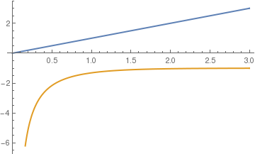
The solution of the differential equation \( y'' + \lambda\,y =0 \) may have one of three forms, depending on λ, so it is necessary to consider these cases. Let us start with λ = 0, the general solution becomes a linear function
If λ is negative, we can let λ = -μ² so that μ > 0. Then the differential equation for y becomes
Next consider λ > 0, then the general solution is
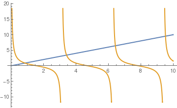
To find the expansion for f in terms of the eigenfunctions, we write
Riemann--Lebesgue Lemma
Bessel's inequality shows that for any square integrable function f ∈ 𝔏²([0, ℓ], ρ), the series
Convergence
Formula \eqref{EqOrtho.7} tells us that there is a mapping
It is most natural to consider pointwise convergence, where we examine the discrepancy at every point. It is difficult (may be impossible) to provide general results about pointwise convergence for general orthogonal functions, but for Fourier series a lot has been done. We have to ask that f(x) be a lot smoother than just belonging to 𝔏², which is a "big" space of functions. You might think having f(x) continuous would be enough, but that obviously does not work at Gibbs phenomenon shows. Here is a slightly different statement of the conditions copied from Keener:
If function f(x) has continuous first derivatives on the interval, except possibly at a finite number of points at which there is a jump in f(x), where left and right derivatives must exist. Then the Fourier series of f converges to ½(f(x+)+f(x−)) for every point in the open interval (0,ℓ). At x=0 and ℓ, the series converges to ½(f(0+)+f(ℓ−)).
The most remarkable result regarding pointwise convergence almost everywhere was obtained by Hans Rademacher (1922) and Dmitrii Menshov (1923).
Another form of convergence is uniform convergence. This used to be the gold standard of convergence. For continuous functions, you can measure the maximum difference between the series and the function written:
Where Do Orthogonal Functions Come From?
The first thing to be looked at is the Gram-Schmidt process.
=================================================
Orthogonal Expansions
There are significant differences between the behavior of Fourier- and power-series expansions. A power series is essentially an expansion about a point, using only information from that point about the function to be expanded (including, of course, the values of its derivatives). We already know that such expansions only converge within a radius of convergence defined by the position of the nearest singularity. However, a Fourier series (or any expansion in orthogonal functions) uses information from the entire expansion interval, and therefore can describe functions that have “nonpathological” singularities within that interval. However, we also know that the representation of a function by an orthogonal expansion is only guaranteed to converge in the mean. This feature comes into play for the expansion of functions with discontinuities, where there is no unique value to which the expansion must converge. However, for Fourier series, it can be shown that if a function f(x) satisfying the Dirichlet conditions is discontinuous at a point x0, its Fourier series evaluated at that point will be the arithmetic average of the limits of the left and right approaches.
- Huaien Li and David C. Torney, A complete system of orthogonal step functions, Proceedings of the American Mathematical Society, 132, No 12, 2004, pp. 3491--3502.
- Menchoff, D.E., (1923), "Sur les séries de fonctions orthogonales. (Première Partie. La convergence.).", Fundamenta Mathematicae (in French), 4: 82–105, doi:10.4064/fm-4-1-82-105
- Rademacher, Hans (1922), "Einige Sätze über Reihen von allgemeinen Orthogonalfunktionen", Mathematische Annalen, Springer Berlin / Heidelberg, 87: 112–138, doi:10.1007/BF01458040
- Titchmarsh, E.C., Eigenfunction Expansions Associated with Second-order Differential Equations. Part I (1946); 2nd. edition (1962).
- Titchmarsh, E.C., Eigenfunction Expansions Associated with Second-order Differential Equations. Part II (1958).
- J. L. Walsh, A closed set of normal orthogonal functions, American Journal of Mathematics, 45, (1923), 5--24.
Return to Mathematica page
Return to the main page (APMA0340)
Return to the Part 1 Matrix Algebra
Return to the Part 2 Linear Systems of Ordinary Differential Equations
Return to the Part 3 Non-linear Systems of Ordinary Differential Equations
Return to the Part 4 Numerical Methods
Return to the Part 5 Fourier Series
Return to the Part 6 Partial Differential Equations
Return to the Part 7 Special Functions