Return to computing page for the first course APMA0330
Return to computing page for the second course APMA0340
Return to computing page for the fourth course APMA0360
Return to Mathematica tutorial for the first course APMA0330
Return to Mathematica tutorial for the second course APMA0340
Return to Mathematica tutorial for the fourth course APMA0360
Return to the main page for the first course APMA0330
Return to the main page for the second course APMA0340
Return to the main page for the fourth course APMA0360
Return to Part V of the course APMA0340
Introduction to Linear Algebra with Mathematica

Glossary

Preface

Our presentation of Fourier series in this section is not done in great depth or generality to meet the pure mathematician's criteria for accuracy. For example, we mostly utilize classical Riemann integration in the majority of examples rather than modern Lebesgue's one in order to make all concepts friendly accessible.

Our exposition is intended as a shop window for basic ideas, techniques, and elegant results of Fourier analysis, with suggested references for further study. The process of understanding is always facilitated if more complicated structures are known to be synthesized from simpler.

Although there are many methods for function representations, Fourier analysis involving the resolution of analog and digital signals into sinusoidal components dominates. Periodic functions occur in a wide range of physical phenomena, a few examples of which are acoustic and electromagnetic waves, periodic vibrations of musical instruments, vertical displacement of a mechanical pendulum, and periodic signals in electrical engineering devices. From theoretical or mathematical point of view, a Fourier series of a function is its spectral decomposition with respect to orthogonal basis formed by eigenfunctions corresponding to a Sturm--Liouville problem.

Sturm--Liouville Problems

Let us start with the regular Sturm--Liouville problem for the first order differential equation subject to the periodic condition,

\[ \hat{p}\,u = %L_1 \left[ \texttt{D} \right] u = \mu\, u(x) \qquad \Longleftrightarrow \qquad {\bf j}\,u' + \mu\, u(x) =0, \qquad u(-\ell ) = u(\ell ) , \]

where the momentum operator \( \hat{p} = -{\bf j}\,\texttt{D} = -{\bf j}\,{\text d}/{\text d}x \) is the first order self-adjoint differential operator containing the imaginary unit j or ⅉ (along the positive vertical direction on the complex plane ℂ), so ⅉ² = −1. As usual, we use Lagrange's notation for the derivative: \( \quad y' = {\text d}y/{\text d}x . \) The formulated problem contains a parameter μ, and it asks to determine the values of the parameter for which the problem has nontrivial (not identically zero) solutions. Such values of parameter μ are referred to as eigenvalues, and the corresponding solutions are called eigenfunctions.

A function 𝑓(𝑥) of one real variable 𝑥 is said to be periodic with period T > 0 if the domain 𝐷(𝑓) of 𝑓 contains 𝑥 + T and 𝑥 − T whenever it contains 𝑥 and if for every 𝑥 ∈ 𝐷(𝑓), it is true that 𝑓(𝑥+T) = 𝑓(𝑥−T) = 𝑓(𝑥).

It follows that if T is a period of 𝑓, then mT is also a period for every integer m > 0. The smallest value of T for which 𝑓(𝑥+T) = 𝑓(𝑥−T) = 𝑓(𝑥) holds is called the fundamental period of 𝑓.

The general solution of the differential equation \( \quad {\mathbf j}\,u'(x) + \mu\, u(x) =0 \quad \) is \( \quad C\,e^{{\bf j}\mu x} , \ \) for some constant C ≠ 0. To satisfy the periodic boundary condition, we have to set μ = nπ/ℓ for some integer n ∈ ℤ = { 0, ±1, ±2, …}. So the eigevalues for this first order differential equation are \( \quad \mu_n = \frac{n\pi}{\ell} = n\,\frac{\pi}{\ell} , \quad n = 0, \pm 1, \pm 2, \ldots , \quad \) to which correspond eigenfunctions \( \quad u_n (x) = e^{{\bf j}\pi n x/\ell} , \quad \) up to some nonzero constant multiple.

Instead of the first order differential operator \( \quad \hat{p} = -{\bf j}\,\texttt{D} = -{\bf j}\,{\text d}/{\text d}x \quad \) with complex coefficient j, it is convenient to square it to obtain \( \quad L_2 [\texttt{D}] = \hat{p}^2 = - \texttt{D}^2 \quad \) in order to get rid of the imaginary unit. This leads to the corresponding Sturm--Liouville problem with a parameter λ:

\[ L_2 \left[ \texttt{D} \right] y = \lambda\,y(x) \qquad \Longleftrightarrow \qquad y'' +\lambda\,y(x) = 0 , \qquad y(-\ell ) = y(\ell ) , \quad y'(-\ell ) = y'(\ell ) , \]

where λ is a non-negative number and \( L_2 \left[ \texttt{D} \right] = - \texttt{D}^2 = \left( -{\bf j}\texttt{D} \right)^2 = \left( \hat{p} \right)^2 \quad \) is the second order differential operator with \( \ \texttt{D} = {\text d}/{\text d}x . \ \) In physics, this operator is called Hamiltonian and it is denoted by Ĥ. The problem assumes that its solution y(x) is a real-valued function defined on a symmetric interval (chosen for simplicity, without any loss of generality) of length T = 2ℓ. Because of periodic boundary conditions, the function y(x) can be considered only on this finite interval, assuming that y(x + T) = y(x) for all x ∈ ℝ. As it was shown in the openning section, the self-adjoint operator \( \quad L_2 \left[ \texttt{D} \right] = - \texttt{D}^2 \quad \) has an infinite discrete set of non-negative eigenvalues \( \ \lambda_k = \left( \frac{k\pi}{\ell} \right)^2 , \quad k=0,\pm 1, \pm 2,\ldots ; \quad \) therefore, L₂ is called a non-negative operator.

Since the differential operator L₂ is a square of of the first order momentum operator \( \quad L_2 \left[ \texttt{D} \right] = \hat{p}^2 , \quad \) its eigenvalues must be squares of the latter:

\[ \lambda_k = \left( \frac{k\pi}{\ell} \right)^2 = \mu_k^2 , \qquad k=0, \pm 1, \pm 2, \ldots . \]

Therefore, eigenvalues λ_k = λ_−k collide for positive and negative indices. However, their eigenfunctions don't, and we have the sequence of real-valued eigenfunctions:

\[ \phi_k (x) = \cos \left( k\,\frac{\pi}{\ell}\,x \right) , \quad k=0,1,2,\ldots ; \qquad \phi_{-k} (x) = \sin \left( \frac{k\pi x}{\ell} \right) , \quad k=1,2,\ldots . \]

Often, eigenfunctions are organized in two-dimensional vector form:

\[ \left\{ \left[ \begin{array}{c} 1 \\ 0 \end{array} \right] , \ \left[ \begin{array}{c} \cos \left( \frac{\pi x}{\ell} \right) \\ \sin \left( \frac{\pi x}{\ell} \right) \end{array} \right] , \ \left[ \begin{array}{c} \cos \left( \frac{2\pi x}{\ell} \right) \\ \sin \left( \frac{2\pi x}{\ell} \right) \end{array} \right] , \ \left[ \begin{array}{c} \cos \left( \frac{3\pi x}{\ell}\right) \\ \sin \left(\frac{3\pi x}{\ell}\right) \end{array} \right] , \cdots \left[ \begin{array}{c} \cos \left(\frac{n\pi x}{\ell}\right) \\ \sin \left(\frac{n\pi x}{\ell}\right) \end{array} \right] , \cdots \right\} . \]

The Sturm--Liouville problems formulated above can be written in operator form

\[ L \left[ \texttt{D} \right] y = \lambda\,y , \qquad y(-\ell ) = y(\ell ) , \]

where L is one of the following differential operators:

\[ L_2 \left[ \texttt{D} \right] = - \texttt{D}^2 \qquad \mbox{or} \qquad \hat{p} = -{\bf j}\,\texttt{D} , \qquad\mbox{with} \quad \texttt{D} = {\text d}/{\text d}x . \]

Actually, these two differential operators are related:

\[ L_2 \left[ \texttt{D} \right] = \left( \hat{p} \right)^2 \qquad \mbox{or} \qquad - \texttt{D}^2 = \left( - {\bf j}\,\texttt{D} \right)^2 = {\bf j}^2 \texttt{D}^2 , \qquad {\bf j}^2 = -1. \]

As it was shown in the previous section, the unbounded linear operator L₂ with periodic condition is a non-negative operator, meaning that all its eigenvalues are not negative.

Any eigenvalue problem can be written in abstract form as \( \quad L\, y = \lambda\,y , \ \) which is actually a spectral representation of the linear operator L. The idea of such representation is to reduce action of the operator L on a function by multiplication operation. In contrast to finite dimensional case (matrices), an unbounded operator has infinite many (maybe continuous) eigenvalues.

Assuming λ≥0, we solve the Sturm--Liouville problem for L₂.

\[ y'' + \lambda\,y = 0, \qquad y(-\ell ) = y(\ell ) \quad y'(-\ell ) = y'(\ell ) . \]

The general solution of the differential equation depends on two arbitrary real constants c₁ and c₂:

\[ y(x) = c_1 \cos \left( \sqrt{\lambda}\,x \right) + c_2 \sin \left( \sqrt{\lambda}\,x \right) . \]

This function can be periodic with period T if and only if

\[ \sqrt{\lambda} = \frac{2\pi n}{T} \qquad \Longrightarrow \qquad \lambda_n = \left( \frac{2\pi n}{T} \right)^2 , \quad n=0,1,2,\ldots . \]

It is a custom to set the period to be an even number: T = 2ℓ. Then due to periodicity of the problem, it is also convenient to consider a symmetric interval [−ℓ, ℓ] because any interval of length T = 2ℓ can be used.

The first order differential operator \( \hat{p} \) acts on complex-valued functions (as well as on real-valued functions). The general solution of \( {\bf j}\,u' + \mu\, u = 0 \) depends on one arbitrary complex number A = 𝑎 + jb (where 𝑎 and b are real numbers):

\[ u(x) = A\, e^{{\bf j}\mu x} = \left( a + {\bf j}b \right) e^{{\bf j}\mu x} = \left( a + {\bf j}b \right) \left( \cos \mu x + {\bf j}\,\sin \mu x \right) . \]

The function u(x) is a periodic function (independently on A) when

\[ \mu = \mu_n = \frac{n2\pi}{T} , \qquad n= 0,\pm 1, \pm 2,\ldots . \]

Note that since \( L_2 \left[ \texttt{D} \right) = \left( -{\bf j}\,\texttt{D} \right)^2 , \) their eigenvalues are related

\[ \lambda_n = \mu_n^2 = \left( \frac{2\pi n}{T} \right)^2 , \quad n=0,\pm 1, \pm 2,\ldots . \]

Finally, we get a sequence of eigenfunctions corresponding to eigenvalues μ_n:

\[ u_n (x) = A_n e^{2{\bf j}n\pi x/T} , \qquad \mbox{where} \quad T = 2\ell . \]

﹡ ⁎ ✱ ✲ ✳ ✺ ✻ ✼ ✽ ❋

An essential part of the Sturm--Liouville theory includes function expansions with respect to the (infinite) system of eigenfunctions---a complete set for every self-adjoint differential operator of the second order subject to the appropriate boundary conditions. The majority of applications of the Sturm--Liouville theory utilizes expansions of a function f(x) that satisfies the homogeneous boundary conditions (in our case, they are periodic conditions)

\begin{equation} \label{EqFourier.1} f(x) \.\sim\, \sum_k c_k \phi_k (x) , \end{equation}

where ϕₖ(x) are eigenfunctions for either second order operator \( \quad L_2 \left[ \texttt{D} \right] = - \texttt{D}^2 \ \) or momentum operator \( \quad \hat{p} = - {\bf j} \texttt{D} . \ \) The sign ∼ indicates that this series was obtained in a purely formal manner. It is replaced by "=" when the series converges to function 𝑓(𝑥), The coefficients cₖ = cₖ(f) of the expansion, \( f(x) = \sum_k \, c_k \,\phi_k (x) , \) for a function f(x) over the set of eigenfunctions {ϕ_k(x)} are called the Fourier coefficients. An ordered list of Fourier coefficients can be considered as a vector in infinite dimensional space spanned on eigenfunctions. We prefer to use Dirac's's notation for identification of this discrete list of Fourier coefficients:

\[ \vert\, f \,\rangle = \left[ \cdots , c_{-n} , \cdots , c_0 , c_1 , c_2 , \cdots , c_n , \cdots \right] . \]

Since every eigenfunction ϕₖ(x) in decomposition \eqref{EqFourier.1} satisfies the periodic condition, we expect that the function f(x) also matches this condition, so we require that f(−ℓ) = f(ℓ). Anyway, the Fourier expansion \eqref{EqFourier.1} assigns numerical values at endpoints for f(x). If the values of f(x) at the endpoints do not match, then this just means that there is a discontinuity at that point---don't worry, the Fourier series will correct you. Hence, the Fourier series, if it converges, dictates the determination of f at endpoints according to the average of its one sided limits:

\[ f(-\ell ) = f(\ell ) = \frac{1}{2} \left[ f(-\ell +0) + f(\ell -0) \right] = \lim_{\varepsilon \downarrow 0} \ \frac{1}{2} \left[ f(-\ell +\varepsilon ) + f(\ell -\varepsilon ) \right] . \]

In many applications, particular values of f(x) at endpoints do not matter because function f(x) is specified on an open interval (−ℓ, ℓ) rather than closed interval. Actually, the Fourier series (if it converges) assigns numerical values at every point of the closed interval [−ℓ, ℓ], including endpoints. Pointwise convergence of series \eqref{EqFourier.1} is discussed in convergence section and other issues of convergence in mean convergence section.

Definition of Fourier Series

Historically, Legendre expansions were first introduced by Adrien‑Marie Legendre in 1784 in his work on the gravitational attraction of ellipsoids. However, it was Joseph Fourier who first claimed, in 1807, that "every function" can be expanded into a series of trigonometric functions. It was later discovered that this claim is valid only for certain classes of functions. Nevertheless, the Fourier series provided the first example of an expansion in terms of eigenfunctions of a Sturm--Liouville problem with periodic boundary conditions.

Since a function represented by a Fourier series must satisfy these boundary conditions, we restrict our attention to periodic functions. Moreover, without loss of generality, we assume that all periodic functions have period T = 2ℓ. It therefore suffices to consider real-valued functions f : [−ℓ, ℓ] → ℝ satisfying \( f(-\ell ) = f(\ell ) = \frac{1}{2} \left[ f(-\ell + 0) + f(\ell -0) \right] , \ \) which ensures compatibility with the periodicity condition.

Every expansion can be written in the series form \eqref{EqFourier.1}. Therefore, it consists of two mutually dependent components: the Fourier coefficients { cₖ } and the set of eigenfunctions { ϕₖ }. Mathematicians later proved the existence of eigenvalues and eigenfunctions, since Sturm and Liouville themselves did not provide such a proof, showing that an unbounded self-adjoint second-order differential operator subject to appropriate homogeneous boundary conditions possesses a discrete set of eigenvalues and corresponding eigenfunctions. Reconstructing a function f(x) from its discrete list of Fourier coefficients | f ⟩ is referred to as forming its Fourier series. In other words, the Fourier series of a function f(x) represents its decomposition into periodic waves, one of the most useful concepts in physics that also plays a central role in many branches of engineering. However, reconstructing the function from its Fourier coefficients is an ill-posed problem.

There are two equivalent forms of Fourier series based on two eigenfunction expansions corresponding to the first order operator \( \hat{p} = - {\bf j}\,\texttt{D} \) and the second order operator \( L_2 \left[ \texttt{D} \right] = - \texttt{D}^2 = \left( -{\bf j} \texttt{D} \right)^2 = \left( \hat{p} \right)^2 = \hat{H}(p) . \) The former one provides an eigenfunction expansion in a complex form (or exponential form)

\begin{equation} \label{EqFourier.2} f(x) \,\sim\, \mbox{V.P.}\sum_{n=-\infty}^{\infty} \hat{f}(n)\, e^{n{\bf j} \pi x/\ell} \ = \ \lim_{N\to \infty} \ \sum_{n=-N}^{N} \hat{f}(n)\, e^{n{\bf j} \pi x/\ell} \ = S[f](x) , \end{equation}

where T = 2ℓ is the period and x is a real variable. As usual, j or ⅉ denotes the unit (imaginary) vector on complex plane ℂ, so j² = −1. Here «V.P.» abbreviates the Cauchy principal value (valeur principale de Cauchy in French), which is a regularization of the infinite summation. Since this series may or may not converge, and if it converges, we don't know whether its sum is f(x), we cannot write \( f(x) \,=\, \sum_{n=-\infty}^{\infty} \hat{f}(n)\, e^{n{\bf j} \pi x/\ell} . \quad \) Hence, we use a tilde (∼) instead of equal symbol (=) simply to identify the fact that the Fourier coefficients \( \hat{f}(n) \) are evaluated according to the Euler--Fourier formulas:

\begin{equation} \label{EqFourier.3} \hat{f}(n) = \frac{1}{2\ell} \int_{-\ell}^{\ell} f(x)\, e^{-n{\bf j} \pi x/\ell} \ {\text d} x = \frac{1}{T} \int_{0}^{T} f(x)\, e^{-2n{\bf j} \pi x/T} \ {\text d} x , \qquad n \in \mathbb{Z} = \left\{ 0, \pm 1, \pm 2, \ldots \right\} . \end{equation}

Derivation of these formulas will be given later, in section on orthogonality. This means that the function f(x) is expanded into formal series \eqref{EqFourier.2} that is convenient to denote the latter by S[f]. Since a restoration of the function f(x) from its Fourier coefficients \eqref{EqFourier.3} is an ill-posed problem, a natural definition of two-sided infinite series (that you learnt in calculus)

\[ \sum_{n=-\infty}^{+\infty} \hat{f}(n)\, e^{n{\bf j} \pi x/\ell} \ = \lim_{N.M \to +\infty} \ \sum_{n=-M}^{N} \hat{f}(n)\, e^{n{\bf j} \pi x/\ell} \]

does not work in many cases.

Example 1: We expand the following complex-valued function into exponential Fourier series:

\[ \pi\, e^{{\bf j}\left( \pi -x \right) \alpha} \quad\sim \, \mbox{P.V.}\ \ e^{{\bf j}\alpha\pi} \ 2\sum_{n=-\infty}^{\infty} \, \frac{\sin \left( n + \alpha \right) \pi}{n+\alpha}\, e^{{\bf j}nx} . \]

Indeed, its Fourier coefficients are

\[ \hat{f} (n) = \frac{1}{\pi} \int_{-\pi}^{\pi} \pi\, e^{{\bf j}\left( \pi -x \right) \alpha} \, e^{-{\bf j}nx} {\text d} x = \frac{2\,\sin \left( n+ \alpha \right) \pi}{\left( n + \alpha \right)}\, e^{{\bf j}\alpha\pi} . \]

Simplify[Integrate[Exp[-I*n*x + I*(Pi - x)*alpha], {x, -Pi, Pi}]] Pi/Sin[Pi*alpha]

-((I E^(-I n \[Pi]) (-1 + E^(2 I (alpha + n) \[Pi])))/(alpha + n)) alpha \[Pi]])/(alpha + n)

When α = ½, we have

\[ \pi\, e^{{\bf j}\left( \pi -x \right) /2} = 2\, e^{{\bf j}\pi /2} \sum_{n=-\infty}^{\infty} \frac{\sin \left( n + \frac{1}{2} \right) \pi}{n+\frac{1}{2}}\, e^{{\bf j}nx} . \]

Separation of real and imaginary parts yields

\begin{align*} \Re \pi\, e^{{\bf j}\left( \pi -x \right) /2} &= \pi \sin \left( \frac{x}{2} \right) = -8 \sum_{n\ge 1} \frac{n (-1)^n}{4 n^2 -1} \,\sin (nx) , \\ \Im \pi\, e^{{\bf j}\left( \pi -x \right) /2} &= \pi \cos \left( \frac{x}{2} \right) = 2 - 4 \sum_{n\ge 1} \frac{(-1)^n}{4n^2 -1}\, \cos (nx ) . \end{align*}

Integrate[Sin[x/2]*Sin[n*x], {x, -Pi, Pi}]

(8 n Cos[n \[Pi]])/(1 - 4 n^2)

■

End of Example 1

Another eigenfunction expansion regarding the second order differential operator \( \displaystyle \quad L_2 (\texttt{D}) = - \texttt{D}^2 = - {\text d}^2/{\text d}x^2 \quad \) gives a trigonometric form of Fourier series

\begin{equation} \label{EqFourier.4} f(x) \,\sim\, \frac{a_0}{2} + \sum_{k=1}^{\infty} \left[ a_k \cos \left( \frac{k \pi x}{\ell} \right) + b_k \sin \left( \frac{k \pi x}{\ell} \right) \right] , \end{equation}

where coefficients are defined according to the Euler--Fourier formulas (they were discovered in 1757 by Leonhard Euler many years before Fourier used them in his research):

\begin{align} a_0 &= a_0 (f) = \frac{1}{\ell} \int_{-\ell}^{\ell} f(x)\,{\text d} x , \notag \\ a_k &= a_k (f) = \frac{1}{\ell} \int_{-\ell}^{\ell} f(x)\, \cos \frac{k \pi x}{\ell} \,{\text d} x , \qquad k= 1, 2, 3, \ldots ; \label{EqFourier.5} \\ b_k &= b_k (f) = \frac{1}{\ell} \int_{-\ell}^{\ell} f(x)\, \sin \frac{k \pi x}{\ell} \,{\text d} x , \qquad k= 1, 2, 3, \ldots . \notag \end{align}

The constant coefficient in series \eqref{EqFourier.4} is written in the form 𝑎₀/2 for convenience to keep all Euler--Fourier formulas \eqref{EqFourier.5} uniform.

Series \eqref{EqFourier.4} is also understood in the Cauchy principal value sense because generally speaking it should be written as

\[ f(x) \,\sim \frac{a_0}{2} + \lim_{N\to +\infty} \ \sum_{k=1}^{N} \, a_k \,\cos \left( \frac{k \pi x}{\ell}\right) + \lim_{M\to +\infty} \ \sum_{k=1}^{M} \,b_k \,\sin \left( \frac{k \pi x}{\ell} \right) . \]

Here the principal value means that M = N.

Sometimes, it is convenient to use polar form:

\[ f(x) \,\sim\, \frac{a_0}{2} + \sum_{k=1}^{\infty} \ A_k \,\sin \left( \frac{k \pi x}{\ell} + \phi_k \right) = \frac{a_0}{2} + \sum_{k=1}^{\infty} \ A_k \,\cos \left( \frac{k \pi x}{\ell} - \varphi_k \right) , \]

where \( A_k = \sqrt{a_k^2 + b_k^2} \quad \) is the wave amplitude, \( \quad \varphi_k = \arctan \left( b_k / a_k \right) , \quad \phi_k = \arctan \left( a_k / b_k \right) \ \) is the phase; and kπ/ℓ is the wave number (or angular frequency), where the wavelength is ℓ/(2k). Therefore, the Fourier series is a way of expressing a function as a sum, or linear superposition of waves of different frequencies that are referred to as modes.

For any real x and integrable on interval [−ℓ, ℓ] function f, we denote by S[f] the Fourier series generated by function f(x) either in trigonometric form

\[ S[f] (x) = \frac{a_0}{2} + \mbox{P.V.} \sum_{k\ge 1} \left[ a_k \,\cos \left( \frac{k \pi x}{\ell} \right) + b_k \,\sin \left( \frac{k \pi x}{\ell} \right) \right] \]

or in complex exponential form

\[ S[f] (x) = \mbox{P.V.} \sum_{k=-\infty}^{+\infty} \,\hat{f}(n)\, e^{{\bf j}n \pi x/\ell} , \]

where coefficients 𝑎ₖ, bₖ and \( \displaystyle \quad \hat{f}(n) \ \) are evaluated according to the Euler--Fourier formulas (5) and (3), respectively.

Note: The definition above did not specify what integrability definition is in use. There are many integrals besides the Riemann and Lebesgue integrals. Most were invented to solve specific problems where Riemann integration fails or where Lebesgue integration is either too weak or unnecessarily general. Fourier analysis actually uses several of them—but Lebesgue integration including Lebesgue–Stieltjes integrals became the standard because it provides the best balance of generality, simplicity, and powerful convergence theorems. Sometimes the requirement that function 𝑓 is absolutely integrable in Lebesgue sense is too restrictive for existence of 𝑆[𝑓] and could be dropped, especially when you deal with improper Riemann integrable functions and distributions.

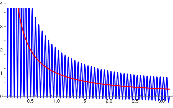
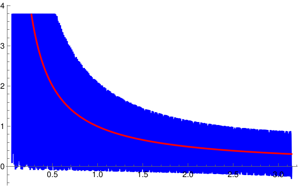
Example 2: Function 𝑓(𝑥) = 1/𝑥 is not absolutely integrable on [0, π], so it does not belong to the Lebesgue space 𝔏¹: \[ \int_0^{\pi} \,\left\vert \frac{1}{x} \right\vert {\text d}x = \int_0^{\pi} \,\frac{{\text d}x}{|x|} = \infty . \] However, its Fourier coefficients exist: \[ b_n = \frac{2}{\pi}\,\int_0^{\pi} \,\frac{\sin (nx)}{x}\,{\text d}x = \frac{2}{\pi}\,\mbox{Si}(n\pi) , \] where Si(𝑥) is the Sine Inetgral, \[ \mbox{Si}(x) = \int_0^x \,\frac{\sin t}{t}\,{\text d}t . \] Hence one formally obtains the Fourier series \[ \frac{1}{x} \,\sim\,\frac{2}{\pi}\,\sum_{n=1}^{\infty}\,\mbox{Si}(n\pi )\,\sin (nx) . \] Now we utilize Mathematica to plot sine Fourier partial sums.

coef = (2/Pi) Table[SinIntegral[n Pi], {n, 500}]; Sfast[x_] := coef.Table[Sin[n x], {n, 500}]; Plot[ {Sfast[x], 1/x}, {x, 0.05, Pi}, PlotStyle -> {{Blue, Thick}, {Red,Thick}}, PlotLegends -> {"Partial sum", "1/x"} ]

Fourier approximation with 100 terms		Fourier approximation with 500 terms

■

End of Example 2

Example 3: Let us consider two functions that can be used to generate saw-tooth graphs. One of them is the absolute value function (on a finite interval) and another one is just its shift:

\[ |x| \qquad \mbox{and} \qquad f(x) = \begin{cases} \ell -x, & \ \mbox{for} \quad 0 \le x < \ell , \\ \ell + x , & \ \mbox{for} \quad -\ell < x \le 0. \end{cases} \]

Using Mathematica, we find Fourier coefficients for the absolute value function.

Assuming[L > 0, Integrate[Abs[x]*Cos[n*Pi*x/L], {x, -L, L}]]

(2 L^2 (-1 + Cos[n \[Pi]] + n \[Pi] Sin[n \[Pi]]))/(n^2 \[Pi]^2)

Assuming[L > 0, Integrate[Abs[x], {x, -L, L}]]

L^2

\[ a_n (|x|) = \frac{1}{\ell} \int_{-\ell}^{\ell} |x|\,\cos \left( \frac{n\pi x}{\ell} \right) {\text d} x = \frac{2\ell}{n^2 \pi^2} \left( (-1)^n -1 \right) = - \frac{4\ell}{(2k-1)^2 \pi^2} , \qquad n=2k-1. \]

Then we use another command

Assuming[L > 0, FourierTrigSeries[Abs[x], x, 5, FourierParameters -> {1, Pi/L}]]

Therefore we get its Fourier series:

\[ |x| = \frac{\ell}{2} - \frac{4\ell}{\pi^2} \sum_{k\ge 1} \frac{1}{(2k-1)^2}\,\cos \left( \frac{\pi \left( 2k-1 \right) x}{\ell} \right) . \]

		We plot with Mathematica: s20[x_] = 1/2 - (4/Pi^2)Sum[Cos[kPix]/(2k - 1)^2, {k, 1, 20}]; Plot[{Abs[x], s20[x]}, {x, -1.2, 1.2}, PlotStyle -> Thick]
Absolute value function and its 20 term Fourier approximation.		Mathematica code

Now we calculate Fourier coefficients for function f(x)

Assuming[L > 0, Integrate[(L - x)*Cos[n*Pi*x/L], {x, 0, L}]/L] + Assuming[L > 0, Integrate[(L + x)*Cos[n*Pi*x/L], {x, -L, 0}]/L]

-((2 L (-1 + Cos[n \[Pi]]))/(n^2 \[Pi]^2))

This allows us to build the corresponding Fourier series

\[ f(x) = \frac{\ell}{2} + \frac{4\ell}{\pi^2} \sum_{k\ge 1} \frac{1}{(2k-1)^2}\,\cos \left( \frac{\pi \left( 2k-1 \right) x}{\ell} \right) . \]

		We plot with Mathematica: s20[x_] = 1/2 + (4/Pi^2)Sum[Cos[kPix]/(2k - 1)^2, {k, 1, 20}]; f[x_] = Piecewise[{{1 + x, x < 0}, {1 - x, x > 0}}]; Plot[{f[x], s20[x]}, {x, -1.2, 1.2}, PlotStyle -> Thickness[0.01]]
Function f(x) and its 20 term Fourier approximation.		Mathematica code

		We plot with Mathematica 50 term approximation to its conjugate Fourier series (which is very close to sine function): \[ S^{\ast} [f](x) = \frac{4\ell}{\pi^2} \sum_{k\ge 1} \frac{1}{(2k-1)^2}\,\sin \left( \frac{\pi \left( 2k-1 \right) x}{\ell} \right) . \] s50[x_] = (4/Pi^2)Sum[Sin[kPix]/(2k - 1)^2, {k, 1, 50}]; Plot[{(4/Pi^2)Sin[Pix], s50[x]}, {x, -1.2, 1.2}, PlotStyle -> Thickness[0.01]]
Function f(x) and its 20 term Fourier approximation.		Mathematica code

■

End of Example 3

A derivation of Euler--Fourier formulas \eqref{EqFourier.3} and \eqref{EqFourier.5} are given in section devoted to orthogonal expansions.

The complex Fourier series \eqref{EqFourier.2} is more elegant and shorter to write down than the one expressed in terms of sines and cosines \eqref{EqFourier.4}, but it has the disadvantage that the coefficients might be complex numbers even if the given function is real-valued. The trigonometric form is based on Euler's formulas:

\[ \sin \theta = \frac{1}{2{\bf j}} \,e^{{\bf j}\theta} - \frac{1}{2{\bf j}} \,e^{-{\bf j}\theta} = \Im \,e^{{\bf j}\theta} = \mbox{Im} \,e^{{\bf j}\theta}, \qquad \cos \theta = \frac{1}{2} \,e^{{\bf j}\theta} + \frac{1}{2} \,e^{-{\bf j}\theta} = \Re \,e^{{\bf j}\theta} = \mbox{Re} \,e^{{\bf j}\theta}. \]

Here, j is the unit vector in the positive vertical direction on the complex plane ℂ, so j² = −1. Of course, these two decompositions \eqref{EqFourier.2} and \eqref{EqFourier.4} are equivalent when each series \eqref{EqFourier.2} and \eqref{EqFourier.4} converges.

Some representations of functions by trigonometric series was first considered by Leonhard Euler in 1753:

\begin{align*} \sum_{n\ge 1} \,\frac{(-1)^n}{n} \,\sin (nx ) &= \frac{x}{2} , \qquad |x| < \pi , \\ \sum_{n\ge 1} \,\frac{(-1)^n}{n^2} \,\cos (nx ) &= \frac{\pi^2}{12} - \frac{x^2}{4} , \qquad |x| < \pi . \end{align*}

Later, Daniel Bernoulli while working on spring vibrations obtained (according to Hobson) more examples of trigonometric series:

\begin{align*} \sum_{n\ge 1} \,\frac{1}{n} \,\sin (nx ) &= \frac{\pi -x}{2} , \qquad 0 < x < 2\pi , \\ \sum_{n\ge 1} \,\frac{1}{n^2} \,\cos (nx ) &= \frac{\pi^2}{6} - \frac{1}{2}\,\pi x + \frac{x^2}{4} , \\ \sum_{n\ge 1} \,\frac{1}{n^3}\,\sin (nx) &= \frac{1}{6}\,\pi^2 x - \frac{\pi}{4}\, x^2 + \frac{x^3}{12} , \qquad 0 < x < 2\pi , \\ \sum_{n\ge 1} \,\frac{1}{n^4} \,\cos (nx ) &= \frac{\pi^4}{90} - \frac{\pi^2}{12}\,x^2 + \frac{\pi}{12}\,x^3 - \frac{x^4}{48}, \qquad 0 \le y \le 2\pi , \\ \sum_{n\ge 1} \,\frac{1}{n^5}\,\sin (nx) &= \frac{\pi^4}{90}\,x - \frac{\pi^2}{36}\,x^3 + \frac{\pi}{48}\, x^4 - \frac{x^5}{240} . \end{align*}

However, neither the greatest mathematician of the eighteenth century, Euler, nor other researchers, including D. Bernoulli and Legendre, recognized these series as particular examples of orthogonal expansions. At the time, the necessary mathematical framework had not yet been developed; for example, the first modern and rigorous definition of a function was given by Peter Dirichlet in 1837. The rigorous mathematical theory of orthogonal expansions emerged only in the early twentieth century (1900–1935). It was Joseph Fourier (1768--1830) who, in 1807, proposed that "any function" could be expanded into a trigonometric series.

Joseph Fourier was arrested in July 1794 during the Reign of Terror because of his political activities and his defense of political rivals in Orléans. After the fall of Maximilien Robespierre, who was executed by guillotine on 28 July 1794, the political situation changed, and Fourier was released from prison on 11 August 1794. Having narrowly escaped execution during the French Revolution, Fourier subsequently turned his attention to an academic career, which was far safer than political life. He became one of the first students at the newly founded École Normale. The following year, he was appointed a teacher there and soon afterward joined the faculty of the École Normale, where he worked alongside Monge and Lagrange.

In 1798, Fourier accompanied Napoleon Bonaparte on his Egyptian expedition as a scientific adviser and was appointed secretary of the Institut d'Égypte. During his stay in Egypt, he contributed several mathematical papers to the Institut, which Napoleon had established in Cairo.

In 1801, Napoleon appointed Fourier Prefect (Governor) of the Department of Isère in Grenoble, where he supervised road construction and numerous other public works. After returning from the Egyptian expedition, Fourier intended to resume his academic position at the École Polytechnique. Napoleon, however, overruled his plans, remarking that Fourier's administrative talents would be of greater service to France.

In a memorable session of the French Academy of Sciences on 21 December 1807, a 39-year-old politician from Grenoble, nearly 600 km from Paris, with few scientific credentials—his papers published in the Mémoires sur l'Égypte were little known in Paris—presented his memoir to the Institute of France. As expected, Fourier's unpublished manuscript, Théorie de la propagation de la chaleur dans les solides, was met with skepticism by several senior members of the Academy, including the great analyst Lagrange.

Fourier claimed that an arbitrary function defined on a finite interval could always be represented as a sum of sine and cosine functions. The academicians had good reason to question this remarkable assertion. Every finite combination of sines and cosines is an infinitely differentiable (indeed, analytic) function, and at the time there was no rigorous theory explaining how an infinite trigonometric series could converge to a function that was not analytic, or even discontinuous.

Subsequent investigations demonstrated that Fourier's claim was entirely justified, although he himself was not able to provide the exact proofs demanded, because the corresponding theory, called after Sturm (1803--1855) and Liouville (1809--1882) appeared only thirty years later.

==============================================

It is well-known that partial Fourier sums display in general a rather irregular behavior as the number of terms grows to infinity. In 1900, Lipót Fejér discovered that the Cesàro means (which is an extension of regular summation method) of the partial sums display a strikingly simpler behavior. This broadened the validity of the Fourier series to a much larger class of functions that does not demand more than mere integrability of functions, without adding any other restrictions concerning continuity or differentiability.

This becomes clear in 1899 when Willard Gibbs reported a phenomenon of conditionally convergent Fourier series that now bare his name. Actually, it was known 50 years before to Henry Wilbraham (1825--1883).
🔶 ❖ ﹡ ⁎ ✱ ✲ ✳ ✺ ✻ ✼ ✽ ❋ ❖ 🔶

Fourier's Impact

Fourier uses his mathematics with the delighful freedom mostly because he did not get a solid background studying math during one year. Nevertheless, he put a lot of efforts to catch up the material during his teaching experience and selfeducation.

Fourier dissertation (and successive monograph publication in 1822) initiated further development in mathematics. First of all, the cornerstone concept of function was establish. Before Fourier's discovery, functions were considered either by analytic formula or geometrically if they could be drawn with the hand. Daniel Bernoulli (1700--1782) believed that any functions can be defined by a formula.

In the later development of mathematics, evaluation of Fourier coefficients requres a proper definition of integrability that was successfully addressed by Bernhard Riemann (1826--1866). He developed a concept of " Riemann-integrability" in 1854, but not published in a journal until 1868. Even this definition was not sufficient for the more abstract speculations of modern mathematics and was once more generalized by Émile Borel (1871--1956) and Henri Lebesgue (1875--1941), who in 1904 extending the applicability of the Fourier series to a still larger class of functions.

It took more than a century for mathematician to develop a rigorous theory of Sturm--Liouville theory and corresponding orthogonal expansions, including summability methods for series.

In 1902, Jacques Salomon Hadamard (1865--1963) introduced definition of well-posed problem. Correspondingly, a problem that is not well-posed, is called ill-posed. It turns out that restoration of a function from its set of Fourier coefficients is an ill-posed problem.

Change of Scale

Coefficient evaluations in the Euler--Fourier formulas \eqref{EqFourier.3} and \eqref{EqFourier.5} can be obtained upon integration over any interval of length T = 2ℓ because of periodically condition. Sometimes it is convenient to consider a function on interval [0,T] (or any interval of length T). Let f(x) be a periodic function over the range 0 ≤ x < T. Then its Fourier series becomes

\[ f(x) \,\sim\, \frac{a_0}{2} + \sum_{k\ge 1} \left[ a_k \cos \left( \frac{2k \pi x}{T} \right) + b_k \sin \left( \frac{2k \pi x}{T} \right) \right] , \tag{4} \]

where coefficients are defined as

\[ \left[ \begin{array}{c} a_k \\ b_k \end{array} \right] = \frac{2}{T} \int_{0}^{T} f(x) \left[ \begin{array}{c} \cos \left( \frac{2\pi kx}{T} \right) \\ \sin \left( \frac{2\pi kx}{T} \right) \end{array} \right] {\text d} x , \qquad k= 0, 1, 2, 3, \ldots . \tag{5} \]

A similar expression is valid for exponential Fourier series.

In general, a square integrable function f ∈ 𝔏²([𝑎, b]) on the interval [𝑎, b] of positive length b−𝑎 (b>𝑎) can be expanded into the Fourier series

\begin{equation} \label{EqFourier.6} f(x) \,\sim\, \frac{a_0}{2} + \sum_{k=1}^{\infty} \left[ a_k \cos \left( \frac{2\pi k (x - a)}{b-a} \right) + b_k \sin \left( \frac{2\pi k (x - a)}{b-a} \right) \right] , \end{equation}

where

\begin{align} a_k &= \frac{2}{b-a} \int_a^b f(x) \,\cos \left( \frac{2\pi k(x - a)}{b-a} \right) {\text d}x , \qquad k=0,1,2,\ldots , \notag \\ \label{EqFourier.7} \\ b_k &= \frac{2}{b-a} \int_a^b f(x) \,\sin \left( \frac{2\pi k(x - a)}{b-a} \right) {\text d}x , \qquad k=1,2,\ldots . \notag \end{align}

Example 4: Consider a function f(x) = x² on the interval [0,2]. Its Fourier coefficients can be determined with Mathematica:

Integrate[x^2, {x, 0, 2}]

8/3

Simplify[Integrate[x^2 * Cos[n*Pi*x], {x, 0, 2}], Assumptions -> Element[n, Integers]]

4/(n^2 \[Pi]^2)

Simplify[Integrate[x^2 * Sin[n*Pi*x], {x, 0, 2}], Assumptions -> Element[n, Integers]]

4/(n \[Pi])

Therefore, we get the following Fourier series for function x²:

\[ x^2 = \frac{4}{3} + \sum_{n\ge 1} \left[ \frac{4}{n^2 \pi^2}\,\cos \left( n\pi x \right) - \frac{4}{n\,\pi}\,\sin \left( n\pi x \right) \right] . \]

Next we plot some partial sums along with the given function x²

S10[x_] = 4/3 + Sum[4/n^2/Pi^2 *Cos[n*Pi*x] - 4/n/Pi*Sin[n*Pi*x], {n, 1, 10}];
S20[x_] = 4/3 + Sum[4/n^2/Pi^2 *Cos[n*Pi*x] - 4/n/Pi*Sin[n*Pi*x], {n, 1, 20}];
S100[x_] = 4/3 + Sum[ 4/n^2/Pi^2 *Cos[n*Pi*x] - 4/n/Pi*Sin[n*Pi*x], {n, 1, 100}];
Plot[{x^2, S10[x]}, {x, -0.5, 2.5}, PlotStyle -> {{Thick, Red}, {Blue, Thick}}] Plot[{x^2, S20[x]}, {x, -0.5, 2.5}, PlotStyle -> {Thick, {Black, Orange}}]
Plot[{x^2, S100[x]}, {x, -0.5, 2.5}, PlotStyle -> {Thick, {Black, Blue}}]

Fourier approximation with 10 terms		Fourier approximation with 100 terms

Now we expand the given function f(x) = x² into complex Fourier series \eqref{EqFourier.2}:

\[ x^2 = \frac{4}{3} + \mbox{P.V.}\,\sum_{n\ne 0} \left( \frac{2}{n^2 \pi^2} + \frac{2{\bf j}}{n\pi} \right) e^{n{\bf j}\pi x} . \]

Integrate[x^2 *Exp[-n*I*Pi*x], {x, 0, 2}]/2

(E^(-2 I n \[Pi]) (-2 I + 2 I E^(2 I n \[Pi]) + 4 n \[Pi] + 4 I n^2 \[Pi]^2))/(2 n^3 \[Pi]^3)

Integrate[x^2 *Exp[-0*I*Pi*x], {x, 0, 2}]/2

4/3

■

End of Example 4

Example 5: We expand the sine function into Fourier series for different values of parameter ℓ that defines the interval from which a function is periodically expanded.

Example 5A: Let us start with ℓ = π. Then sinx itself is its Fourier series; so no work is required.

Example 4B: For ℓ = π/2, we get Fourier coefficients

\[ \hat{f} (n) = \frac{1}{\pi} \int_{-\pi /2}^{\pi /2} \sin x\, e^{-n{\bf j}2x} {\text d}x = \frac{4n{\bf j}}{\left( 4n^2 -1 \right) \pi} \left( -1 \right)^n , \qquad n = 0, \pm 1, \pm2 , \ldots . \]

Integrate[Sin[x]*Exp[-n*I*2*x], {x, -Pi/2, Pi/2}]/Pi

(4 I n Cos[n \[Pi]])/((-1 + 4 n^2) \[Pi])

This provides the exponential Fourier series of sine function:

\[ \sin x = \mbox{P.V.} \frac{1}{\pi} \sum_{n=-\infty}^{\infty} \frac{4n{\bf j}}{4n^2 -1} \left( -1 \right)^n e^{{\bf j}2nx} . \]

Fourier coefficients for trigonometric series are

\[ a_k = \frac{2}{\pi} \int_{-\pi /2}^{\pi /2} \sin x\, \cos \left( 2k x \right) {\text d} x = 0 0 \]

and

\[ b_k = \frac{2}{\pi} \int_{-\pi /2}^{\pi /2} \sin x\, \sin \left( 2k x \right) {\text d} x = \frac{8k}{\left( 1 - 4k^2 \right) \pi} \, (-1)^k . \]

We plot the corresponding approximations with 15 and 50 term.

S15[x_] = (8/Pi)*Sum[n/(1 - 4*n^2 )*(-1)^n * Sin[2*n*x], {n, 1, 15}];
Plot[{Sin[x], S15[x]}, {x, -Pi, Pi}, PlotStyle -> Thick]
S50[x_] = (8/Pi)*Sum[n/(1 - 4*n^2 )*(-1)^n * Sin[2*n*x], {n, 1, 50}];
Plot[{S50[x]}, {x, -Pi, Pi}, PlotStyle -> Thick]

Fourier approximation with 15 terms		Fourier approximation with 50 terms

Example 5C: For ℓ = π/3, we get Fourier coefficients

\[ \hat{f} (n) = \frac{3}{2\pi} \int_{-\pi /3}^{\pi /3} \sin x\, e^{-n{\bf j}3x} {\text d}x = \frac{9\sqrt{3}n{\bf j}}{\left( 9n^2 -1 \right) 2\pi} \left( -1 \right)^n , \qquad n = 0, \pm 1, \pm2 , \ldots . \]

Integrate[Sin[x]*Exp[-n*I*3*x], {x, -Pi/3, Pi/3}]*(3/2/Pi)

(3 I (3 Sqrt[3] n Cos[n \[Pi]] - Sin[n \[Pi]]))/(2 (-1 + 9 n^2) \[Pi])

This provides the exponential Fourier series of sine function on interval (−π/3, π/3):

\[ \sin x = \frac{9\sqrt{3}}{2\pi} \sum_{n=-\infty}^{\infty} \frac{n{\bf j}}{9n^2 -1} \left( -1 \right)^n e^{{\bf j}3nx} . \]

Fourier coefficients for trigonometric series are

\[ a_k = \frac{3}{\pi} \int_{-\pi /3}^{\pi /3} \sin x\, \cos \left( 3k x \right) {\text d} x = \]

and

\[ b_k = \frac{3}{\pi} \int_{-\pi /3}^{\pi /3} \sin x\, \sin \left( 3k x \right) {\text d} x = -\frac{9\sqrt{3}\,k}{\left( 9 \k^2 -1 \right) \pi} \left( -1 \right)^k , \qquad k=1,2,3,\ldots . \]

Integrate[Sin[x]*Cos[k*3*x], {x, -Pi/3, Pi/3}]*(3/Pi)

Integrate[Sin[x]*Sin[k*3*x], {x, -Pi/3, Pi/3}]*(3/Pi)

(3 (-3 Sqrt[3] k Cos[k \[Pi]] + Sin[k \[Pi]]))/((-1 + 9 k^2) \[Pi])

We plot the corresponding approximations with 12 and 55 term.

S12[x_] = (9*Sqrt[3]/Pi)* Sum[n/(1 - 9*n^2)*(-1)^n*Sin[3*n*x], {n, 1, 12}];
Plot[{Sin[x], S12[x]}, {x, -Pi, Pi}, PlotStyle -> Thick]
S55[x_] = (9*Sqrt[3]/Pi)* Sum[n/(1 - 9*n^2)*(-1)^n*Sin[3*n*x], {n, 1, 55}];
Plot[{S55[x]}, {x, -Pi, Pi}, PlotStyle -> Thick]

Fourier approximation with 12 terms		Fourier approximation with 55 terms

■

End of Example 5

Harmonic functions

Fourier series and corresponding formulas become much easier to handle upon introducing the new variable ϑ = π·x/ℓ. Let us consider the series of the form

\begin{equation} \label{EqFourier.8} f(\vartheta ) \,\sim\, \frac{a_0}{2} + \sum_{k=1}^{\infty} \left[ a_k \cos \left( k\vartheta \right) + b_k \sin \left( k\vartheta \right) \right] , \end{equation}

where ϑ is a real variable and coefficients 𝑎₀, 𝑎ₖ, bₖ, … are independent of ϑ and real. The factor ½ in the constant term will be found to be a convenient convention.

Series \eqref{EqFourier.8} is known as the trigonometric series. The series are formal series: there is no implication of their convergence for all or any ϑ at this moment. Actually, the trigonometric series above is written in the Cauchy principal value form because it is the sum of two series

\[ \frac{a_0}{2} + \sum_{k=1}^{\infty} \left[ a_k \cos \left( k\vartheta \right) + b_k \sin \left( k\vartheta \right) \right] = \frac{a_0}{2} + \sum_{k=1}^{\infty} a_k \cos \left( k\vartheta \right) + \sum_{k=1}^{\infty} b_k \sin \left( k\vartheta \right) . \]

Since their convegence cannot be ignored, they are understood as simultaneous limits with the same upper bound:

\[ \sum_{k=1}^{\infty} a_k \,\cos \left( k\vartheta \right) + b_k \,\sin \left( k\vartheta \right) = \lim_{n\to\infty} \ \sum_{k=1}^{n} a_k \,\cos \left( k\vartheta \right) + b_k \,\sin \left( k\vartheta \right) . \]

The Cauchy principal form allows us to unite these two series into one, containing a complex parameter. Let cₙ = ½(𝑎ₙ − jbₙ), where j, also denoted as ⅉ, is the imaginary unit, so ⅉ² = −1. Using Euler's formula \( \displaystyle \quad e^{\mathbf{j}\vartheta} = \cos\vartheta + \mathbf{j}\,\sin\vartheta , \quad \) we rewrite the general term as

\[ a_n \cos n\vartheta + b_n \sin n\vartheta = \frac{a_n}{2} \left( e^{\mathbf{j}\,n\vartheta} + e^{-\mathbf{j}\,n\vartheta} \right) + \frac{b_n}{2\mathbf{j}} \left( e^{\mathbf{j}\,n\vartheta} - e^{-\mathbf{j}\,n\vartheta} \right) . \]

Collecting common terms, we obtain

\[ a_n \cos n\vartheta + b_n \sin n\vartheta = \frac{1}{2}\, e^{\mathbf{j}\,n\vartheta} \left( a_n - \mathbf{j}\,b_n \right) + \frac{1}{2}\, e^{-\mathbf{j}\,n\vartheta} \left( a_n + \mathbf{j}\,b_n \right) . \]

Upon setting \[ c_n = \frac{1}{2} \left( a_n - \mathbf{j}\,b_n \right) , \quad b_0 = 0, \quad a_{-n} = a_n , \quad b_{-n} = - b_n , \quad n > 0, \] we obtain the series that is equivalent to \eqref{EqFourier.8}:

\begin{equation} \label{EqFourier.9} f(\vartheta ) \,\sim\, \mbox{V.P.}\, \sum_{n=-\infty}^{\infty} \, c_n e^{\mathbf{j}\,n\vartheta} , \qquad c_n = \frac{1}{2} \left( a_n - \mathbf{j}\,b_n \right) = \left( c_{-n} \right)^{\ast} , \end{equation}

where c^✶ is complex conjugate to c. This series is also called the trigonometric series in complex form. If coefficients 𝑎ₙ, bₙ and cₙ are evaluated via the Euler--Fourier formulas

\begin{align*} a_k &= \frac{1}{\pi} \int_{-\pi}^{\pi} f(x) \,\cos \left( k\vartheta \right) {\text d}x , \qquad k=0,1,2,\ldots , \\ & \qquad \tag{5} \\ b_k &= \frac{1}{\pi} \int_{-\pi}^{\pi}\, f(x) \,\sin \left( k\vartheta \right) {\text d}x , \qquad k=1,2,\ldots . \end{align*}

and

\[ c_n = \hat{f} (n) = \frac{1}{2\pi}\,\int_{-\pi}^{\pi}\, f(t)\, e^{-\mathbf{j}nt} \ {\text d} t , \qquad n=0,\pm 1, \pm 2, \ldots . \tag{3} \]

then the series \eqref{EqFourier.8} or \eqref{EqFourier.9} is called the Fourier series.

The question of whether every trigonometric series is the Fourier series of a function has played a central role in the historical development of Fourier analysis. During the nineteenth century, this problem remained unresolved and stimulated extensive research into the convergence and representation of trigonometric series. It is now known that the answer is negative in general: not every trigonometric series is the Fourier series of a function within the classical function spaces. Nevertheless, for several important classes of functions, necessary and sufficient conditions have been established that determine whether a given trigonometric series is the Fourier series of a function belonging to the class under consideration. These characterizations constitute a fundamental aspect of the theory of Fourier series and illustrate the close relationship between the analytical properties of functions and the behavior of their Fourier coefficients.

Example 6: There are cases when the trigonometric series is given by its coefficients but we do not know whether it is a Fourier series of a certain function or not.

In order to support our claim that not every trigonometric series is a Fourier series, we are going to provide an example. First what comes to anybody mind is a divergence series, say \[ \frac{1}{2} + \sum_{n\ge 1} \ \cos (nt) . \] This series cannot define an ordinary function. Indeed, for any fixed 𝑡,

it 𝑡 = 0, every cosine equals 11, so the series diverges to +∞+∞;
If 𝑡 ≠ 2πk, the partial sums oscillate and do not converge.

Thus the series has no pointwise meaning as a function.

However, this series weak converges (in distribution sense) to the 2π-periodic a href="https://en.wikipedia.org/wiki/Dirac_delta_function">Dirac delta function.

For every smooth 2π-periodic test function 𝑓, \[ \int_{-\pi}^{\pi}\ \left( \frac{1}{2} + \sum_{n\ge 1} \ \cos (nt) \right) f(t) \,{\text d}t = \pi\,f(0) . \] This is exactly the defining action of πδ_2π(t)πδ2π(𝑡). So if you're working with Fourier series on a 2π-periodic interval, the correct identity is \[ \frac{1}{2} + \sum_{n\ge 1} \ \cos (nt) = \pi\,\delta_{2\pi} (t) . \]

Hence, we are forced to consider the case when Coefficients growing too fast. For instance, let \[ c_n = e^{\sqrt{|n|}} , \] then \[ \sum_{n=-\infty}^{\infty} \ c_n\,e^{\mathbf{j}\,nx} \] cannot be the Fourier series of any distribution, since Fourier coefficients of periodic distributions satisfy \[ \left\vert c_n \right\vert = O\left( n^m \right) \] for some m. This series is non-Fourier in the strongest possible sense, although admittedly less interesting analytically because it fails a simple growth condition. ■

End of Example 6

In what follows \( \displaystyle \quad z = x + \mathbf{j}\,y = r\,e^{\mathbf{j}\vartheta} \quad \) is a complex variable and \( \displaystyle \quad \overline{z} = z^{\ast} = x - \mathbf{j}\,y = r\,e^{-\mathbf{j}\vartheta} \quad \) is its conjugate. Note that we prefer using asterisk notation for complex conjugate vs overline. To fix our ideas, we suppose 𝑎ₙ and bₙ to be real numbers (so that cₙ and c₋ₙ are conjugate).

The trigonometric series \eqref{EqFourier.8} is the real part of the series

\[ F(z) = \frac{1}{2}\, a_0 + \sum_{n\ge 1}\left( a_n - \mathbf{j}\,b_n \right) z^n , = c_0 + 2\,\sum_{n\ge 1} \, c_n z^n , \qquad z = e^{\mathbf{j}\vartheta} , \]

when z belongs to the unit circle. However, this series defines a holomorphic function inside the disk |z| < 1:

\[ F\left( r\,e^{\mathbf{j}\vartheta} \right) = \frac{1}{2}\, a_0 + \sum_{n\ge 1}\left( a_n - \mathbf{j}\,b_n \right) \, r^n \, e^{\mathbf{j}n\vartheta} = u(r, \vartheta ) + \mathbf{j}\,v(r, \vartheta ) , \]

where

\begin{equation} \label{EqFourier.10} \begin{split} u(r, \vartheta ) &= \frac{1}{2}\, a_0 + \sum_{n\ge 1}\left( a_n\,\cos n\vartheta + b_n\,\sin n\vartheta \right) \, r^n , \\ v(r, \vartheta ) &= \sum_{n\ge 1}\left( a_n\,\sin n\vartheta - b_n\,\cos n\vartheta \right) \, r^n . \end{split} \end{equation}

Example 7: We consider the signum function \[ \mbox{sign} (t) = \begin{cases} \phantom{-}1, &\qquad \mbox{for } t > 0 , \\ \phantom{-}0, &\qquad t = 0, \\ -1, &\qquad \mbox{for } t < 0 . \end{cases} \] It is odd, so its Fourier series contains only sine terms. \[ \mbox{sign}(t) = \sum_{n\ge 1} b_n \,\sin (nt) , \] where \[ b_n = \frac{2}{\pi}\,\int_0^{\pi} \,\sin (nx)\,{\text d}x = \frac{2}{n\pi} \left( 1 + (-1)^n \right) . \]

(2/Pi)*Integrate[Sin[n*x], {x, 0, Pi}]

(2 (1 - Cos[n \[Pi]]))/(n \[Pi])

Thereore, \[ \mbox{sign}(\vartheta ) = \frac{4}{\pi}\,\sum_{k\ge 1} \ \frac{\sin (2k-1)\vartheta}{2k-1} . \] Now we compute the complex Fourier coefficients: \[ c_n = \frac{1}{2}\left( a_n - \mathbf{j}\,b_n \right) = - \frac{\mathbf{j}}{2}\,b_n \] This yields \[ c_{2k} = 0, \qquad c_{2k-1} = - \frac{2\mathbf{j}}{\pi\left( 2k-1 \right)} \] Now we construct the analytic function. The analytic function is obtained from the positive frequencies: \[ F(z) = 2\,\sum_{n\ge 1} c_n \,z^n = - \frac{4\mathbf{j}}{\pi}\,\sum_{k\ge 1}\ \frac{z^{2k-1}}{2k-1} . \] Fortunately, Mathematica recognizes this sum as the Taylor expansion of arctangent:

Sum[z^(2*k - 1) /(2*k - 1), {k, 1, Infinity}]

ArcTanh[z]

\[ \mbox{arctan}(z) = \sum_{k\ge 1} \ \frac{z^{2k-1}}{2k-1} , \qquad |z| < 1 . \] Hence, \[ F(z) = - \frac{4\mathbf{j}}{\pi}\,\mbox{arctan}(z) . \] Equivalently, \[ F(z) = - - \frac{2\mathbf{j}}{\pi}\,\ln \left( \frac{1+z}{1-z} \right) , \qquad |z| < 1 , \] where the principal branch of the logarithm is used. We need to compute the real and imaginary parts of F(z). Since \[ \ln w = \ln |w| + \mathbf{j}\,\mbox{arg} w , \] we get \[ u(r, \vartheta ) = \Re \,F(z) = \frac{2}{\pi}\,\mbox{arg} \left( \frac{1 + r\,e^{\mathbf{j}\,\vartheta}}{1 - r\,e^{\mathbf{j}\,\vartheta}} \right) , \] and \[ v (r, \vartheta ) = - \frac{2}{\pi}\,\ln \left\vert \left( \frac{1 + r\,e^{\mathbf{j}\,\vartheta}}{1 - r\,e^{\mathbf{j}\,\vartheta}} \right) \right\vert . \] Using \[ \left\vert 1 \pm r\,e^{\mathbf{j}\,\vartheta} \right\vert^2 = 1 + r^2 \pm 2r\,\cos\vartheta , \] this expression becomes \[ v (r, \vartheta ) = - \frac{2}{\pi}\,\ln \left( \frac{1 + r^2 + 2r\,\cos\vartheta}{1 + r^2 - 2r\,\cos\vartheta} \right) . \] For the real part, one convenient expression is \[ u (r, \vartheta ) = \frac{4}{\pi}\,\mbox{arctan} \left( \frac{2r\,\sin\vartheta}{1-r^2} \right) . \] where the appropriate branch of arctan is chosen so that u is continuous for r<1.

As r → 1, we have \[ u (r, \vartheta ) \to \mbox{sign}(\vartheta ) \] for every continuity point of 𝑓, while \[ v (r, \vartheta ) \to -\frac{2}{\pi}\,\ln \left\vert \tan\frac{\vartheta}{2} \right\vert . \] Thus, the Hilbert transformation of u(1, ϑ) is \[ \mathcal{H}\,\mbox{sogn}(\vartheta ) = -\frac{2}{\pi}\,\ln \left\vert \tan\frac{\vartheta}{2} \right\vert . \] This logarithmic function is the periodic Hilbert transform of the sign function

Finally, we check that functions u(r, ϑ) and v(r, ϑ) are harmonic functions, that is, they satisfy the Laplace equation. To accomplish this task, we emply Mathematica.

u[r_, t_] = (4/Pi)*ArcTan[2*r*Sin[t] /(1 - r^2)]; (1/r)*D[r*D[u[r, t], r], r] + D[u[r, t], t, t]/r^2 FullSimplify[%]

and

v[r_, t_] = (2/Pi) * Log[(1 + r^2 + 2*r*Cos[t])/(1 + r^2 - 2*r*Cos[t])] (1/r)*D[r*D[v[r, t], r], r] + D[v[r, t], t, t]/r^2 FullSimplify[%]

Therefore, these two functions are harmonic functions: \[ \frac{1}{r}\,\frac{\partial}{\partial r} \left( r\,\frac{\partial u}{\partial r} \right) + \frac{1}{r^2} \,\frac{\partial^2 u}{\partial r^2} = 0, \qquad \frac{1}{r}\,\frac{\partial}{\partial r} \left( r\,\frac{\partial v}{\partial r} \right) + \frac{1}{r^2} \,\frac{\partial^2 v}{\partial r^2} = 0 . \] ■

End of Example 7

If Fourier coefficients are bounded (which we always assume), then the series

\[ u(r, \vartheta ) = \,\mbox{V,P,} \sum_{-\infty}^{\infty} \, c_n r^{|n|} e^{n\mathbf{j}\vartheta}\, =\, \frac{a_0}{2} + \sum_{n\ge 1} r^n \left( a_n \cos (n\vartheta ) + b_n \sin (n\vartheta ) \right) \]

converges for 0 ≤ r < 1 and for a fixed r, uniformly in ϑ. The Cauchy–Riemann equations imply that both functions, u(r, ϑ) and v(r, ϑ), are harmonic functions, i.e., solutions of the homogeneous Laplace equation

\[ \left( r\,\frac{\partial}{\partial r} \right)^2 u + \frac{\partial^2 u}{\partial \vartheta^2} = 0 , \qquad \left( r\,\frac{\partial}{\partial r} \right)^2 v + \frac{\partial^2 v}{\partial \vartheta^2} = 0 . \]

Example 8: Let us consider the holomorphic function \[ F(z) = \frac{1+z}{1-z} , \] which maps the unit disk conformally onto the right half-plane. Let z = r (cosϑ + ⅉ sinϑ), 0 ≤ r < 1. Then \[ F(z) = \frac{1 + r\,e^{\mathbf{j}\,\vartheta}}{1 - r\,e^{\mathbf{j}\,\vartheta}} . \] Multiply numerator and denominator by conjugate of the denominator to make it real, we get \[ \left( 1 + r\,e^{\mathbf{j}\,\vartheta} \right) \left( 1 - r\,e^{-\mathbf{j}\,\vartheta} \right) = 1 - r^2 + 2\mathbf{j}\,r\,\sin\vartheta . \] Hence, \[ F \left( r\,e^{\mathbf{j}\,\vartheta} \right) = \frac{1- r^2}{1 - 2r\,\cos\theta + r^2} + \mathbf{j}\,\frac{2r\,\sin\vartheta}{1 - 2r\,\cos\theta + r^2} = u + \mathbf{j}\,v . \] where \[ u = \frac{1- r^2}{1 - 2r\,\cos\theta + r^2} , \qquad v = \frac{2r\,\sin\vartheta}{1 - 2r\,\cos\theta + r^2} . \] So u is the Poisson kernel and v is the conjugate Poisson kernel.

Let us consider when r → 1−0. The real part is zero, while the total integral remains \[ \frac{1}{2\pi}\,\int_{-\pi}^{\pi} \,u(r,\vartheta )\,{\text d}\vartheta = 1 . \] Thus, \[ u(r,\vartheta ) \to 2\pi\,\delta (\vartheta ) \qquad\mbox{as } \ r\to 1 , \] in the distributional sense. The imaginary part \[ v(r, \vartheta ) \to \cos\frac{\vartheta}{2} \qquad\mbox{as } \ r\to 1 , \] again in the principal value sense. This is precisely the kernel of the periodic Hilbert transform.

Expand \[ F(z) = 1 + 2\,\sum_{n\ge 1} \ z^n \] Substituting \( \displaystyle \quad z = r\,e^{\mathbf{j}\,\vartheta} ,\quad \) we have \[ F\left( r\,e^{\mathbf{j}\,\vartheta} \right) = 1 + 2\sum_{n\ge 1}\ r^n\,e^{\mathbf{j}\,n\vartheta} . \] This function has a simple form \[ F\left( r\,e^{\mathbf{j}\,\vartheta} \right) = 1 + \frac{2\,r\,e^{\mathbf{j}\,\vartheta}}{1 - r\,e^{\mathbf{j}\,\vartheta}} = \frac{1 + r\,e^{\mathbf{j}\,\vartheta}}{1 - r\,e^{\mathbf{j}\,\vartheta}} \]

Sum[r^n *Exp[I*n*t], {n, 1, Infinity}]

-((E^(I t) r)/(-1 + E^(I t) r))

Therefore, separating real and imaginary parts, we obtain \[ u(r, \vartheta ) = 1 + 2\,\sum_{n\ge 1} \ r^n \cos (n\vartheta ) = \frac{1- r^2}{1 - 2r\,\cos\theta + r^2} , \] and \[ v(r, \vartheta ) = 2\,\sum_{n\ge 1} \ r^n \sin (n\vartheta ) = \frac{2r\,\sin\vartheta}{1 - 2r\,\cos\theta + r^2} . \] This immediately shows that v is obtained from u by replacing each cosine mode with the corresponding sine mode, illustrating the harmonic conjugation underlying the periodic Hilbert transform.

■

End of Example 8

The functions u(r, ϑ) and v(r, ϑ) of Eq.(10) are called conjugate harmonic functions, and the series (with zero constant term and ϑ = π·x/ℓ), corresponding to v(1, ϑ)

\begin{align*} S^{\ast}[f] (x) &= \sum_{k\ge 1} \left[ a_k \sin \left( \frac{k \pi x}{\ell} \right) - b_k \cos \left( \frac{k \pi x}{\ell} \right) \right] \\ &= \mbox{P.V.} \left( -{\bf j} \right) \sum_{n=-\infty}^{+\infty} \left( \mbox{sign}\, n \right) \hat{f}(n)\, e^{{\bf j}n \pi x /\ell} , \qquad \hat{f}(n) = \frac{1}{2\ell} \,\int_{-\ell}^{\ell}\, f(x)\, e^{-\mathbf{j}\,\pi nx/\ell;;}\,{\text d}x , \end{align*}

is called the conjugate Fourier series. The coefficients 𝑎ₖ, bₖ and \( \displaystyle \quad \hat{f}(n) \quad \) are defined by the Euler--Fourier formulas (5) and (3), respectively.

The Hilbert transform of function 𝑓(𝑥), 𝑥 ∈ ℝ, is defined by the convolution integral

\[ \mathcal{H}\,f(x) = \frac{1}{\pi x} \ast f = \mbox{V.P.}\,\frac{1}{\pi}\,\int_{\mathbb{R}}\,\frac{f(t)}{x-t}\,{\text d}t= \mbox{V.P.}\,\frac{1}{\pi}\,\int_{\mathbb{R}}\,\frac{f(x-t)}{t}\,{\text d}t , \]

where the convolution is understood in the principal value sense. When function 𝑓(𝑥) is 2π-periodic, the kernel 1/𝑥 is replaced by sum of all integer translates:

\[ \sum_{k \in \mathbb{Z}} \ \frac{1}{\theta + 2k\pi} = \frac{1}{2}\,\cot \,\frac{\theta}{2} . \]

The kernel of Hilbert's transformation has Fourier series

\[ \frac{1}{2}\,\cot \,\frac{\theta}{2} = \mbox{V.P.}\,\sum_{n\ne 0} \left( -\mathbf{j}\,\mbox{sign}(n) \right) e^{\mathbf{j}n\theta} , \]

in the sense of distributions. The Hilbert transform acting on 2ℓ-periodic function is defined by

\[ \left( \mathcal{H}_{\ell} f \right) (x) = \frac{1}{2\ell} \,\mbox{V.P.} \int_{-\ell}^{\ell} \,f(t)\,\cot \left( \frac{\pi \left( x-t \right)}{2\ell} \right) {\text d}t = \frac{1}{2\ell} \,\mbox{V.P.} \int_{-\ell}^{\ell} \,f(x-t)\,\cot \left( \frac{\pi t}{2\ell} \right) {\text d}t . \]

When ℓ = π, it is common to drop index ℓ in the definition of of the Hilbert transform:

\[ \left( \mathcal{H}\,f \right) (\vartheta ) = \frac{1}{2\pi} \left( \cot \frac{\vartheta}{2} \right) \ast f = \frac{1}{2\pi} \,\mbox{V.P.} \int_{-\pi}^{\pi} \,f(\vartheta -t)\,\cot \left( \frac{t}{2} \right) {\text d}t , \]

which is exactly the convolution representation corresponding to the Fourier multiplier. Using formulas

\[ \mathcal{H}_{\ell}\left( \cos \frac{n\pi x}{\ell} \right) = \sin \frac{n\pi x}{\ell} , \qquad \mathcal{H}_{\ell}\left( \sin \frac{n\pi x}{\ell} \right) = -\cos \frac{n\pi x}{\ell} , \]

we apply the Hilbert transformation ℋ_ℓ to the Fourier series \( \displaystyle \quad S[f](x) = \frac{a_0}{2} + \sum_{n\ge 1} \ a_n\,\cos \frac{n\pi x}{\ell} + b_n \,\sin \frac{n\pi x}{\ell} \ \) span> and obtain

\[ \mathcal{H}_{\ell}\left( S[f] \right) = \sum_{n\ge 1}\ \left( a_n\,\sin \frac{n\pi x}{\ell} - b_n \,\cos \frac{n\pi x}{\ell} \right) , \]

which is exactly the conjugate Fourier series. Then, the holomorphic function can be written as

\[ F \left( e^{\mathbf{j}\,\vartheta} \right) = f + \mathbf{j}\,{\mathcal H}\,f = u(1, \vartheta ) + \mathbf{j}\,v(1, \vartheta ) . \]

Example 9: We consider the following piecewise continuous function on interval [0, π] (so 2ℓ = π): \[ f(x) = \begin{cases} \sin (x), \qquad& \mbox{for } \ 0 < x < \pi /2 , \\ \frac{1}{2}\,\cos (x), \qquad & \mbox{for }\ \pi /2 < x < \pi . \end{cases} \] The corresponding Fourier coefficients are \begin{align*} a_0 &= \frac{2}{\pi}\, \int_0^{\pi /2} \, \sin (t)\,{\text d}t + \frac{1}{\pi}\,\int_{\pi /2}^{\pi} \,\cos (t)\,{\text d}t = \frac{1}{\pi} , \\ a_n &= \frac{2}{\pi}\, \int_0^{\pi /2} \, \sin (t)\,\cos (2nt)\,{\text d}t + \frac{1}{\pi} \,\int_{\pi /2}^{\pi} \,\cos (t)\,\cos (2nt) \,{\text d}t = \frac{1}{\pi}\cdot \frac{(-1)^n -2}{4 n^2 -1} , \\ b_n &= \frac{2}{\pi}\, \int_0^{\pi /2} \, f(x)\,\sin (2nx)\,{\text d}x = \frac{1}{\pi}\cdot \frac{2n - 4n\,(-1)^n}{4 n^2 -1} , \qquad n=1,2,\ldots . \end{align*}

f[t_] := Piecewise[{{Sin[t], 0 < t < Pi/2}, {-Cos[Pi - t]/2, Pi/2 < t < Pi}}]; a0 = (2/Pi)*Integrate[f[x], {x, 0, Pi}]

1/\[Pi]

an = (2/Pi)*Integrate[f[t]*Cos[2*n*t], {t, 0, Pi}]

(-2 + Cos[n \[Pi]] + 4 n Sin[n \[Pi]] - 2 n Sin[2 n \[Pi]])/((-1 + 4 n^2) \[Pi])

bn = (2/Pi)*Integrate[f[t]*Sin[2*n*t], {t, 0, Pi}]

(-4 n Cos[n \[Pi]] + 2 n Cos[2 n \[Pi]] + Sin[n \[Pi]])/((-1 + 4 n^2) \[Pi])

Therefore, the Fourier series for function f is \[ S[f] (x) = \frac{1}{2\pi} + \frac{1}{\pi}\,\sum_{n\ge 1} \ \frac{(-1)^n -2}{4 n^2 -1} \, \cos (2nx) + \frac{2n - 4n\,(-1)^n}{4 n^2 -1} \,\sin (2nx) . \] Its complex form becomes \[ S[f] (x) = \frac{1}{2\pi} + \frac{1}{2\pi}\,\sum_{n = -\infty}^{\infty} \ \frac{1}{4 n^2 -1} \left[ \left( (-1)^n -2 \right) - \mathbf{j}\,\left( 2n - 4n\,(-1)^n \right) \right] e^{2\mathbf{j}\,nx} . \]

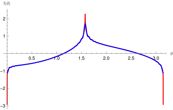
s50[x_] = 1/Pi/2 + (1/Pi)* Sum[((-1)^n - 2)/(4*n^2 - 1) * Cos[2*n*x] + (2*n - 4*n*(-1)^n)/(4*n^2 - 1) * Sin[2*n*x], {n, 1, 50}]; Plot[{f[t], s50[t]}, {t, 0, Pi}, PlotRange -> All, AxesLabel -> {"\[Theta]", "f(\[Theta])"}, PlotStyle -> {{Red, Thick}, {Blue, Thick}}, Exclusions -> {Pi/2}]

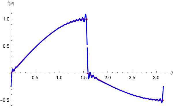
The conjugate Fourier series is \[ S^{\ast}[f] (x) = \frac{1}{\pi}\,\sum_{n\ge 1} \ \frac{(-1)^n -2}{4 n^2 -1} \, \sin (2nx) - \frac{2n - 4n\,(-1)^n}{4 n^2 -1} \,\cos (2nx) \] Now we find the Hilbert transform of the given function f(x): \[ g(x) = \mathcal{H}_{\pi /2} \, f(x) = \frac{1}{\pi} \,\mbox{V.P.}\,\int_0^{\pi /2} \,\sin t\,\cot (x-t)\,{\text d}t + \frac{1}{2\pi} \,\mbox{V.P.}\,\int_{\pi /2}^{\pi} \,\cos t\,\cot (x-t)\,{\text d}t \] The key identity for the first integral is \[ \sin t = \sin x\,\cos (x-t) - \cos x\,\sin (x-t) , \] which gives \[ \sin t\,\cot (x-t) = \sin x \,\frac{\cos^2 (x-t)}{\sin (x-t)} - \cos x\,\cos (x-t) . \] Now use the identity \[ \frac{\cos^2 u}{\sin u} = \frac{1 - \sin^2 u}{\sin u} = \csc u - \sin u . \] Therefore, \[ \sin t\,\cot (x-t) = \sin x\,\csc (x-t) - \sin x\,\sin (x-t) - \cos x\,\cos (x-t) . \] The last two terms combine nicely: \[ -\sin x\,\sin (x-t) - \cos x\,\cos (x-t) = -\cos t , \] so \[ \sin t\,\cot (x-t) = \sin x\,\csc (x-t) - \cos t . \] This is the crucial simplification, which allows us to evaluate the first integral: \[ I_1 = \mbox{V,P.}\,\int_0^{\pi /2} \ \sin t\,\cot (x-t)\,{\text d}t = \sin x\,\int_0^{\pi /2} \ \csc (x-t)\,{\text d}x - \int_0^{\pi /2} \,\cos t\,{\text d}t . \] The latter is just 1. In the singular part, let u = x − t: \[ \mbox{V.P.}\,\int_0^{\pi /2} \ \csc (x-t)\,{\text d}t = \mbox{V.P.}\,\int_{x - \pi /2}^{x} \ \csc u\,{\text d}u = \ln \left\vert \tan \frac{u}{2} \right\vert_{u= x-\pi /2}^x . \] Hence, \[ I_1 = \sin x\,\ln \left\vert \frac{\tan (x/2)}{\tan (x - \pi /2)/2} \right\vert -1 . \] The principal value is automatically encoded by the logarithm.

The second integral is treated similarly, so \[ \cos t = \cos x\,\cos (x-t) + \sin t\,\sin (x-t) , \] which leads to \[ \cos t \,\cot (x-t) = \cos x\,\csc (x-t) + \sin t . \] Therefore, \[ I_2 = \mbox{V.P.}\, \int_{\pi /2}^{\pi} \,\cos t\,\cot (x-t)\,{\text d}t = \cos x\,\mbox{V.P.}\,\int_{\pi /2}^{\pi} \,\csc (x-t)\,{\text d}t + \int_{\pi /2}^{\pi} \,\sin t\,{\text d}t . \] Since \[ \int_{\pi /2}^{\pi} \,\sin t\,{\text d}t = 1, \] we get \[ I_2 = \cos x\,\ln \left\vert \frac{\tan (x - \pi /2)/2}{\tan (x-\pi )/2} \right\vert + 1 . \] Putting everything together, \begin{align*} g(x) &= \frac{1}{\pi}\,I_1 + \frac{1}{2\pi}\,I_2 \\ &= \frac{1}{\pi} \left[ \sin x\,\ln \left\vert \frac{\tan x/2}{\tan (x - \pi /2)/2}| \right\vert -1 \right] + \frac{1}{2\pi} \left[ \cos x\,\ln \left\vert \frac{\tan (x - \pi /2)/2}{\tan (x-\pi )/2}| \right\vert +1 \right] . \end{align*} This expression is valid for 0g(x = ℋ_π/2\,f(x along with 50-term approximation of S^✶[f]:

sast50[x_] = (1/Pi)* Sum[((-1)^n - 2)/(4*n^2 - 1) * Sin[2*n*x] - (2*n - 4*n*(-1)^n)/(4*n^2 - 1) * Cos[2*n*x], {n, 1, 50}]; g[x_] := Sin[x]/Pi *Log[Abs[(Tan[x/2])/(Tan[(x - Pi/2)/2])]] + Cos[x]/(2*Pi) *Log[Abs[(Tan[(x - Pi/2)/2])/(Tan[(x - Pi)/2])]] - 1/(2*Pi); Plot[{g[t], sast50[t]}, {t, 0, Pi}, PlotRange -> All, AxesLabel -> {"\[Theta]", "f(\[Theta])"}, PlotStyle -> {{Red, Thick}, {Blue, Thick}}, Exclusions -> {Pi/2}]

Function 𝑓(𝑥) and its Fourier approxation with 50 terms		Function ℋ𝑓(𝑥) and its conjugate Fourier approximation with 50 terms

■

End of Example 9

Evaluation of Fourier Coefficients

Numerical evaluation of Fourier coefficients becomes a challenging problem for large indices because it leads to integrals with very fast oscillating integrands.

The following formulas could be helpful for evaluations of Fourier coefficients (\( \texttt{D} = \texttt{D}_t = {\text d}/{\text d}t \) is the derivative operator):

Theorem 2:

\begin{align*} \int t^n \cos (at) \,{\text d}t &= - \frac{1}{a} \sum_{k=0}^n \frac{1}{a^k} \, {\texttt D}_t^k \left( t^k \right) \left. {\texttt D}_z^{k+1} \left( \cos z \right) \right\vert_{z=at} \\ &= - \frac{1}{a} \left[ t^n {\texttt D}_z \cos z + \frac{n\,t^{n-1}}{a} \, {\texttt D}_z^2 \cos z + \cdots + \frac{n!}{a^n} \, {\texttt D}_z^{n+1} \cos z \right]_{z=at} , \\ \int t^n \sin (at) \,{\text d}t &= - \frac{1}{a} \sum_{k=0}^n \frac{1}{a^k} \, {\texttt D}_t^k \left( t^k \right) \left. {\texttt D}_z^{k+1} \left( \sin z \right) \right\vert_{z=at} \\ &= - \frac{1}{a} \left[ t^n {\texttt D}_z \sin z + \frac{n\,t^{n-1}}{a} \, {\texttt D}_z^2 \sin z + \cdots + \frac{n!}{a^n} \, {\texttt D}_z^{n+1} \sin z \right]_{z=at} . \end{align*}

Example 15: Let's consider the following half-wave rectifier of the function cosx on interval [−π/2, ;π/2]:

\[ f(x) = \begin{cases} \cos x, & \ \mbox{ when } \ -\frac{\pi}{2} \le x \le \frac{\pi}{2} , \\ 0 , & \ \mbox{ when } \ \frac{\pi}{2} \le x \le \frac{3\pi}{2} . \end{cases} \]

Outside the interval of length 2π, the function f(x) is expanded periodically.

f[t_] = Piecewise[{{Cos[t], -Pi/2 < t < Pi/2}, {0, -Pi < t < -Pi/2 && Pi/2 < t < Pi}}]

Out[1]= { Cos[t] - Pi/2 < t < Pi/2
{ 0 True

Plot[f[t], {t, -Pi, Pi}, PlotStyle -> Thick]

Mathematica will treat the function f[t] outside the interval [-π , π ] as zero

Plot[f[t], {t, -3*Pi, 3*Pi}, PlotStyle -> Thick]

As we see, Mathematica rescales vertical and horizontal lines so that the picture becomes almost symmetric. You can return to the proper picture by using AspectRatio option:

Plot[f[t], {t, -3*Pi, 3*Pi}, PlotStyle -> Thick, AspectRatio -> 1/3/Pi, Ticks -> {True, None}]

So we get exactly the same graph. Now we are ready to expand this function into Fourier series by finding its Fourier coefficients:

\begin{align*} a_0 &= \frac{1}{\pi} \int_{-\pi /2}^{\pi /2} \cos x\,{\text d} x = \frac{2}{\pi} , \\ a_k &= \frac{1}{\pi} \int_{-\pi /2}^{\pi /2} \cos x\, \cos \left( k\, x \right) {\text d} x = -\frac{2}{\pi}\, \frac{1}{k^2 -1} \, \cos \frac{k\pi}{2} , \qquad k= 2, 3, \ldots ; \\ b_k &= \frac{1}{\pi} \int_{-\pi /2}^{\pi /2} \cos x\, \sin \left( k\, x \right) {\text d} x =0, \qquad k= 1, 2, 3, \ldots . \end{align*}

Then the corresponding Fourier series becomes

\[ f(t) \,=\,\frac{1}{\pi} + \frac{1}{2}\, \cos t - \frac{2}{\pi} \, \sum_{k\ge 1} \frac{1}{k^2 -1} \,\cos \left( k\, x \right) . \]

A partial sum with N = 20 terms gives a very good approximation:

Example 16: We consider a piecewise continuous function that cannot be extended into Taylor series because it is identically zero on the interval (1,2). However, we can find its Fourier series.

f[x_] = Piecewise[{{1 - x, 0 < x < 1}, {0, 1 < x < 2}}]

Out[2]= { 1-x, if 0<x<1 and 0 for 1<x<2.

The standard Mathematica command FourierTrigSeries provides you the Fourier series of the function that is extended periodically from the standard interval (-π,π):

FourierTrigSeries[f[x], x, 3]

Out[2]= 1/(4 \[Pi]) + (2 Cos[x] Sin[1/2]^2)/\[Pi] + (Cos[2 x] Sin[1]^2)/(2 \[Pi]) + (2 Cos[3 x] Sin[3/2]^2)/(
9 \[Pi]) + ((2 - 2 Sin[1]) Sin[x])/(2 \[Pi]) - ((-2 + Sin[2]) Sin[2 x])/(4 \[Pi]) - ((-3 + Sin[3]) Sin[3 x])/(9 \[Pi])

With option FourierParameters, it is equivalent to

FourierTrigSeries[f[x], x, 3, FourierParameters -> {1, 1}]

We can plot the partial sum with say 50 terms. Since Fourier partial sums oscillate near points of discontinuity exhibiting so called Gibbs phenomenon, we indicate maximum wiggle (overshoot) and minimum one:

curve = FourierTrigSeries[f[x], x, 50];
Plot[curve, {x, -1.5, 13.5}, PlotRange -> {-0.3, 1.3}, Ticks -> {{Pi, 2*Pi, 3*Pi}, {1.09, -0.09}}, PlotStyle -> Thick]

However, it is not what we want: we need the Fourier series of the function f[x] extended periodically from the interval of length 2:

FourierTrigSeries[f[x], x, 3, FourierParameters -> {1, Pi}]

Out[3]= 1/4 + (2 Cos[\[Pi] x])/\[Pi]^2 + (2 Cos[3 \[Pi] x])/(9 \[Pi]^2) + Sin[\[Pi] x]/\[Pi] + Sin[2 \[Pi] x]/(2 \[Pi]) + Sin[3 \[Pi] x]/( 3 \[Pi])

To check, we find the Fourier coefficients manually:

Integrate[f[x]*Cos[n*Pi*x], {x, 0, 2}, Assumptions -> Element[n, Integers]]

Out[4]= (1 - Cos[n \[Pi]])/(n^2 \[Pi]^2)

\[ a_0 = \frac{1}{2} , \qquad a_n = \frac{1- (-1)^n}{n^2 \pi^2} , \quad n=1,2,\ldots . \]

Integrate[f[x]*Sin[n*Pi*x], {x, 0, 2}, Assumptions -> Element[n, Integers]]

Out[5]= (n \[Pi] - Sin[n \[Pi]])/(n^2 \[Pi]^2)

which is 1/(n*π). Hence, its Fourier series becomes

\[ f(x) = \frac{1}{4} + \sum_{n\ge 1} \left[ \frac{1- (-1)^n}{n^2 \pi^2} \, \cos \left( n \pi x \right) + \frac{1}{n\pi}\, \sin \left( n \pi x \right) \right] \]

We can also represent f(x) in other forms:

\[ f(x) = \frac{1}{4} + \sum_{n\ge 1} \sqrt{ \left( \frac{1- (-1)^n}{n^2 \pi^2} \right)^2 + \frac{1}{n^2 \pi^2}} \, \sin \left( n \pi x + \arctan \frac{1- (-1)^n}{n \pi} \right) = \frac{1}{4} + \sum_{n\ge 1} \sqrt{ \left( \frac{1- (-1)^n}{n^2 \pi^2} \right)^2 + \frac{1}{n^2 \pi^2}} \, \cos \left( n \pi x - \mbox{arccot} \frac{1- (-1)^n}{n \pi} \right) . \]

Now we plot some partial sums, starting with the given function itself:

Plot[f[x], {x, -1, 3}, PlotRange -> {0, 1}, AspectRatio -> Automatic, Axes -> {True, False}, PlotStyle -> Thick]

Then we plot some finite sums:

curve5Pi = FourierTrigSeries[f[x], x, 5];
Plot[%, {x, -1, 3}]

Then we repeat calculations with 50 terms:

Next we plot the correct Fourier series partial sums:

curve5=FourierTrigSeries[f[x], x, 50, FourierParameters -> {1, Pi}];
Plot[%, {x, -1, 3}]

■

There is an elegant application of Fourier series involving Bessel functions:

\[ \cos \left( a\,\sin x \right) = J_0 (a) + \sum_{k\ge 1} J_{2k} (a) \,\cos \left( 2kx \right) . \]

Computing an integral in Mathematica is fairly painless, and it's tempting to simply use a partial Fourier sum depending to the number of terms n. We show how these commands work with several examples.

Mathematica has four default commands to calculate Fourier series:

FourierSeries (* to calculate complex coefficient expansion *)
FourierTrigSeries (* to calculate standard Fourier expansion via sine and cosine *)
FourierCosSeries (* to calculate cosine Fourier series *)
FourierSinSeries (* to calculate sine Fourier series *)

The option FourierParameters has two parameters and when applied, it looks as FourierParameters->{𝑎,b}
In trigonometric form, with setting \( {\bf FourierParameters} \,-> \,\{ a, b \} \) the following series is returned:

\[ \left\vert \frac{b}{\pi} \right\vert^{(1+a)/2} \left[ \frac{a_0}{2} + \sum_{k=1}^n \left( a_k \,\cos (bkt) + b_k \,\sin (bkt) \right) \right] , \]

with

\[ a_k = \left\vert \frac{b}{\pi} \right\vert^{(1+a)/2} \,\int_{-\pi/|b|}^{\pi/|b|} f(t)\,\cos (bkt) \,{\text d}t , \qquad k=0,1,2,\ldots , \]

\[ b_k = \left\vert \frac{b}{\pi} \right\vert^{(1+a)/2} \,\int_{-\pi/|b|}^{\pi/|b|} f(t)\,\sin (bkt) \,{\text d}t , \qquad k=1,2,\ldots . \]

Syntax for the FourierSeries command is: FourierSeries [ function , variable , number of terms ]

Changing the FourierParameters setting allows you to control the limits of integration on the coefficients, and therefore, the base frequency of the series. Some work will go into calculating what value for “b” will give the proper limits of integration. There is ordinarily no reason to change “𝑎” from its default setting, which is 1.

Example 6: We consider a pulse function of length h:

\[ f(x) = \begin{cases} 1 , & \quad\mbox{for} \quad -h/2 < x < h/2 , \\ 0, & \quad\mbox{otherwise}. \end{cases} \]

We expand this function into Fourier series from interval {−ℓ, ℓ], assuming that ℓ > h.

Integrate[Exp[-n*I*Pi*x/L], {x, -h/2, h/2}]/2/L

Sin[(h n \[Pi])/(2 L)]/(n \[Pi])

\[ f(x) = \begin{cases} 1 , & \quad\mbox{for} \quad -h/2 < x < h/2 , \\ 0, & \quad\mbox{otherwise;} \end{cases} = \sum_{n=-\infty}^{+\infty} \frac{1}{n\pi}\,\sin \left( \frac{nh\pi}{2\ell} \right) e^{{\bf j} n\pi x/\ell} . \]

with coefficient corresponding to n = 0 to be \( \displaystyle |\,f\,\rangle = \frac{h}{\2\ell} . \)

Integrate[Cos[n*Pi*x/L], {x, -h/2, h/2}]/L

(2 Sin[(h n \[Pi])/(2 L)])/(n \[Pi])

Integrate[Sin[n*Pi*x/L], {x, -h/2, h/2}]/L

\[ f(x) = \begin{cases} 1 , & \quad\mbox{for} \quad -h/2 < x < h/2 , \\ 0, & \quad\mbox{otherwise;} \end{cases} = \frac{h}{2\ell} + \sum_{n=-1}^{+\infty} \frac{2}{n\pi}\,\sin \left( \frac{nh\pi}{2\ell} \right) \cos \left( \frac{n\pi x}{\ell} \right) . \]

Now setting h = 1 and ℓ = 2, we plot Fourier approximations with 12 and 50 terms.

S12[x_] = 1/4 + Sum[2*Sin[n*Pi/4]*Cos[n*Pi*x/2]/n/Pi, {n, 1, 12}];
f[x_] = Piecewise[{{1, -1/2 < x < 1/2}}];
Plot[{f[x], S12[x]}, {x, -2.5, 2.5}, PlotStyle -> Thick]
S50[x_] = 1/4 + Sum[2*Sin[n*Pi/4]*Cos[n*Pi*x/2]/n/Pi, {n, 1, 50}];
Plot[{S50[x]}, {x, -2.5, 2.5}, PlotStyle -> Thick]

Fourier approximation with 12 terms		Fourier approximation with 55 terms

■

Example 7: We consider the unnormalized sinc function, which is defined by the formula

\[ \mbox{sinc}(x) = \frac{\sin x}{x} . \]

Its Fourier coeffcents

\[ a_k = \frac{1}{\ell} \int_{-\ell}^{\ell} \mbox{sinc}(x) = \frac{\sin x}{x} \,\cos \left( \frac{k\pi x}{\ell} \right) {\text d}x = \frac{1}{\ell} \left[ \mbox{Si} (\ell + n\pi ) + \mbox{Si} (\ell - n\pi ) \right] \]

are expressed through sine integral (a special function):

\[ \mbox{Si}(x) = \int_0^x \frac{\sin t}{t} \,{\text d} t . \]

Integrate[Sin[x]*Cos[n*Pi*x/L]/x, {x, -L, L}]/L

(SinIntegral[L - n \[Pi]] + SinIntegral[L + n \[Pi]])/L

Upon setting ℓ = 2, we plot sinc(x) approximations with 14 and 25 terms.

S12[x_] = SinIntegral[2]/2 + Sum[(SinIntegral[2 - n \[Pi]] + SinIntegral[2 + n*Pi])* Cos[n*Pi*x/2]/2, {n, 1, 12}];
Plot[{Sin[x]/x, S12[x]}, {x, -2.5, 3.5}, PlotStyle -> Thick]
S25[x_] = SinIntegral[2]/2 + Sum[(SinIntegral[2 - n \[Pi]] + SinIntegral[2 + n*Pi])* Cos[n*Pi*x/2]/2, {n, 1, 25}];
Plot[{Sin[x]/x, S25[x]}, {x, -2.5, 3.5}, PlotStyle -> Thick]

Fourier approximation with 12 terms		Fourier approximation with 25 terms

■

Theorem 3: Suppose that \( \left\{ (x_k, y_k ) \right\}_{k=0}^N \) are N+1 points, where \( y_k = f(x_k ) , \) and the abscissas are equally spaced:

\[ x_k = -\ell + \frac{2\ell \,k}{N} \qquad \mbox{for} \quad k=0,1,2,\ldots N. \]

If f(x) is periodic with period \( 2\ell \) and 2M < N, then there exists a trigonometric polynomial

\[ F_M (x) = \frac{a_0}{2} + \sum_{j=1}^M \left[ a_j \cos \left( j\pi x \right) + b_j \sin \left( j\pi x \right) \right] \]

that minimizes the quantity

\[ \sum_{k=1}^N \left\vert f(x_k ) - F_M (x_k ) \right\vert^2 . \]

The coefficients 𝑎_k and b_k of this trigonometric polynomial are computed with the formulas:

\begin{align*} a_j &= \frac{2}{N} \,\sum_{k=1}^N f(x_k ) \,\cos \left( j\,\pi \,x_k \right) \qquad\mbox{for}\quad j=0,1,\ldots , M , \\ b_j &= \frac{2}{N} \,\sum_{k=1}^N f(x_k ) \,\sin \left( j\,\pi\, x_k \right) \qquad\mbox{for}\quad j=1,2,\ldots , M . \qquad\qquad ⧫ \end{align*}

Example 8: Consider the function \( f (x) = x^2 \) on the interval [-1,1]. Let us take 16 equally spaced points \( x_k = -1 + \frac{2k}{15} , \quad k=0,1,2,\ldots , 15. \) Suppose we want to find the trigonometric polynomial approximation for M = 6 to the 15 data points \( \left\{ (x_k, y_k ) \right\}_{k=1}^{15} . \)

Since the periodic extension is assumed, at a point of discontinuity x = 1, the function value f(1) must be computed using the formula

\[ f(1) = \frac{f(1-0) + f(1+0)}{2} = \frac{1+1}{2} =1. \]

The function \( f (x) = x^2 \) is an even continuous function that is extended periodically; hence the coefficients for the sine terms are all zero (i.e. \( b_j =0 \) for all j). The trigonometric polynomial of degree M = 6 involves only the cosine terms, and we get

\[ a_j = \frac{2}{15} \,\sum_{k=1}^{15} \left( \frac{2k}{15} -1 \right)^2 \cos \left( j\,\pi\, x_k \right) \qquad\mbox{for}\quad j=0,1,2,\ldots , 6 . \]

Now we ask Mathematica for help:

Do[a[j_] := (2/15)* Sum[(2*k/15 - 1)^2 *Cos[j*Pi*(2*k/15 - 1)], {k, 1, 15}], {j, 0, 6}]

Then we calculate the trigonometric polynomial and plot it.

C6[x_] := a[0]/2 + Sum[a[j]*Cos[j*Pi*x], {j, 1, 6}]
Plot[{x^2 , FC6[x]}, {x, -1, 1}, PlotRange -> {-0.1, 1}, PlotStyle -> {{Thick, Blue}, {Thick, Orange}}]

As we see from the graph above, a six term approximation gives a relatively good representation of the given function. ■

Discretization

Euler--Fourier formulas \eqref{EqFourier.3} or \eqref{EqFourier.5} provide discretization of a corresponding function f, so they can be considered as transferring a signal into discrete sets:

\[ \vert\,f \,\rangle = \left[ \cdots , \hat{f}(-n) , \cdots , \hat{f}(-1) , \ \hat{f}(0) ,\ \hat{f}(1) ,\cdots , \hat{f}(n) , \cdots \right] \]

\[ \vert\,f \,\rangle = \left( \begin{bmatrix} a_0 \\ 0 \end{bmatrix} , \ \begin{bmatrix} a_1 \\ b_1 \end{bmatrix} \ \begin{bmatrix} a_2 \\ b_2 \end{bmatrix} , \ \begin{bmatrix} a_3 \\ b_3 \end{bmatrix} , \ \cdots \right) = \left[ \cdots , b_k, b_{k-1} , \cdots , b_1 , a_0, a_1 , a_2 , \cdots , a_k , \cdots \right] . \]

Fourier series formulas

\[ f(x) \,\sim\, \mbox{P.V.}\sum_{n=-\infty}^{+\infty} \hat{f}(n)\, e^{n{\bf j} \pi x/\ell} = \lim_{N\to \infty} \sum_{n=-N}^{N} \hat{f}(n)\, e^{n{\bf j} \pi x/\ell} = S[f], \tag{2} \]

\[ f(x) \,\sim\, \frac{a_0}{2} + \sum_{k=1}^{\infty} \left[ a_k \cos \left( \frac{k \pi x}{\ell} \right) + b_k \sin \left( \frac{k \pi x}{\ell} \right) \right] = S[f], \tag{4} \]

provide the inverse transformation from discrete (or digital) form ∣f ⟩ into analog form. Restoration of a function f(x) from its discrete set ∣f ⟩ is an ill-posed problem. It depends not only on properties of the function f(x), but also on the definition of convergence of infinite series.

Example 12: Let us consider a piecewise continuous function

\[ f(x) = \begin{cases} 0, & \ \mbox{ for} \quad -2 < x < 0 , \\ -1/2 , & \ \mbox{ for} \quad x=0, \\ (x-1)^2 , & \ \mbox{ for} \quad 0 < x < 2 . \end{cases} \tag{14.1} \]

■

End of Example 12

Convergence of Fourier Series

Is it true that partial Fourier sums S_N(f; x) converge to the function f(x) as N → ∞? In general, that is far too much to hope for because restoration of a function from its Fourier coefficients ∣f ⟩ is an ill-posed problem. Not every function is suitable for a Fourier series expansion, but those that satisfy some conditions. For example, the tangent function tan(x) cannot be expanded into the Fourier series on any interval containing the roots of the equation cos(x) = 0 simply because the Fourier coefficients do not exist. For certain kinds of functions convergence is assured; but we will see that some functions are so weird that S_N(f; x) diverges for every x.

It was a surprise when the German mathematician Paul David Gustav du Bois-Reymond (1831--1889) was able in 1873 to construct a continuous function whose Fourier series diverges at a point. Despite this negative result, we might ask what happens if we add more smoothness conditions on a generating function. Although we don't know necessary and sufficient conditions for a function to be expanded into a Fourier series, we know some sufficient conditions that guarantee a Fourier series expansion. The Fourier series does not exist unless, for example, 𝑎₀ exists (i.e., \( \left\vert \int_{-\ell}^{\ell} f(x) \,{\text d}x \right\vert < \infty \) ). Even when the integral for 𝑎₀ exists, the Fourier series may converge to another function.

Example 13:

End of Example 11

■

All expansion formulas involve infinite series; their convergence is based on properties of partial sums, either \eqref{EqFourier.2}

\[ S_N (f;x) = \sum_{k=-N}^{N} \hat{f}(k)\, e^{k{\bf j} \pi x/\ell} \tag{6} \]

for complex-valued functions, or \eqref{EqFourier.4}

\[ S_N (f;x) = \frac{a_0}{2} + \sum_{k=1}^{N} \left[ a_k \cos \frac{k \pi x}{\ell} + b_k \sin \frac{k \pi x}{\ell} \right] , \tag{7} \]

for real-valued functions. A Fourier series converges when its partial sums S_N(f; x) approach a limit in some sense; it exists not for arbitrary functions. Since a Fourier series is a series involving trigonometric functions, the corresponding partial sums depend on a parameter x∈ℝ. Upon considering partial sums for every value of x, we arrive at the pointwise convergence of the series of functions (in our case, trigonometric functions). A pointwise convergence of Fourier series is a very delicate matter, which we touch in convergence section.

A natural question that comes to your mind is whether the series \eqref{EqFourier.2} or \eqref{EqFourier.4} converges and if they converge, do they converge to generating function f(x)? Mathematicians tell us that none of these questions have simple answers. We still do not know the exact conditions to fully identify the class of functions whose Fourier series pointwise converge to the same functions. Identification of the function from its Fourier coefficients is an ill-posed problem, and in many cases it requires a regularization. One of such possible regularization is discussed in Cesàro summation section. Nonetheless, Fourier series usually work quite well (especially in situations where they arise from physical problems).

We leave discussion of convergence of Fourier series to two following sections; however, here we use a simple sufficient conditions that is easy to verity.

Theorem 7: Every function from the domain of a self-adjoint differential operator of second order can be expanded into uniformly convergent Fourier series over the set of its eigenfunctions.

The proof of this theorem is based on reduction of the problem to an integral equation. Then using the Hilbert--Schmidt theorem, a function is expanded into series over eigenfunctions. See details in a course on integral equations.

Recall that the domain of a linear differential operator of order n consists of all functions that have continuous derivatives up to the order n and satisfy the differential equation and the boundary conditions that generate the linear operator. Since a Fourier series is an expansion over eigenfunctions of the second order differential operator \( L_2 \left[ \texttt{D} \right] = - \texttt{D}^2 = - {\text d}^2 /{\text d}x^2 , \) subject to the periodic boundary conditions, the domain of L₂ consists of all periodic twice differentiable functions. The equation \( L_2 \left[ \texttt{D} \right] y = \lambda\, y \) to be satisfied requires that the second derivative is also a periodic function.

Theorem 8: If a periodic function f possesses two continuous derivatives, then its Fourier series S[f](x) converges uniformely to f(x).

Remember that a Fourier series is also generated by the first order self-adjoint differential operator \( \hat{p} = - {\bf j}\,\texttt{D} , \) with j being the imaginary unit on ℂ. However, the Sturm--Liouville theory is applicable only to the second order self-adjoint differential operators, and its application to the first order operators requires further development. Nevertheless, we will see later that existence of periodic continuous derivative will be sufficient for convergence of the Fourier series.

Example 14: We consider the the function f(x) = (cosx)⁴ on interval [−π, π]. Expanding it into Fourier series, we get

\[ \cos^4 x = \frac{3}{2} + \frac{1}{2}\,\cos 2x + \frac{1}{8}\,\cos 4x . \]

Integrate[(Cos[x])^4, {x, -Pi, Pi}]/Pi

3/4

Integrate[(Cos[x])^4*Cos[n*x], {x, -Pi, Pi}]/Pi

(2 (24 - 16 n^2 + n^4) Sin[n \[Pi]])/(n (64 - 20 n^2 + n^4) \[Pi])

We check the answer with Mathematica:

S11[x_] = 3/2 + Cos[2*x]/2 + Cos[4*x]/8;
p111 = Plot[{S11[t]}, {t, -\[Pi], \[Pi]}, PlotStyle -> {Thickness[0.02], Purple}];
p112 = Plot[(Cos[t])^4, {t, -\[Pi], \[Pi]}, PlotStyle -> {Thickness[0.007], Blue}];
Show[p111, p112]

■

Operations on Fourier Series

Theorem 11: Let f(x) be an absolutely integrable function on interval [−ℓ, ℓ] and let S[f] be its exponential Fourier series, that is,

\[ f(x) \sim S[f] = \mbox{P.V.} \sum_{n=-\infty}^{+\infty} \hat{f}(n) \, e^{{\bf j}\pi nx/\ell} . \]

Then

\[ \overline{f(x)} \sim \mbox{P.V.} \sum_{n=-\infty}^{+\infty} \overline{\hat{f}(n)} \, e^{-{\bf j}\pi nx/\ell} = \sum_{n=-\infty}^{+\infty} \overline{\hat{f}(-n)} \, e^{{\bf j}\pi nx/\ell} ; \]
\[ e^{{\bf j}\pi mx/\ell} f(x) \sim \mbox{P.V.} \sum_{n=-\infty}^{+\infty} \overline{\hat{f}(n)} \, e^{-{\bf j}\pi \left( n + m \right) x/\ell} = \sum_{n=-\infty}^{+\infty} \hat{f}(n-m)\, e^{{\bf j}\pi nx/\ell} \]
\[ f(x+y) \sim \mbox{P.V.} \sum_{n=-\infty}^{+\infty} \hat{f}(n)\, e^{{\bf j}\pi nx/\ell} \, e^{{\bf j}\pi ny/\ell} . \]

The proofs are simple and straightforward (so we omit them).

Theorem 12: If \( f(x) \sim \sum_{n=-\infty}^{+\infty} \alpha_n e^{{\bf j}\pi nx/\ell} \) and \( g(x) \sim \sum_{n=-\infty}^{+\infty} \beta_n e^{{\bf j}\pi nx/\ell} , \) then

\[ \sum_{n=-\infty}^{+\infty} \alpha_n \beta_n e^{{\bf j}\pi nx/\ell} = \frac{1}{2\ell}\,f\star g (x) = \frac{1}{2\ell} \int_{-\ell}^{\ell} f(x-y)\,g(y) \,{\text d} y . \]

We show first that the convolution integral exists for almost all x. We can assume that functions f and g are real-valued functions. Without any loss of generality, we can assume that both functions are not negative. Then

\[ \int_{-\ell}^{\ell} {\text d}x \int_{-\ell}^{\ell} {\text d} y\, f(x-y)\,g(y) = \int_{-\ell}^{\ell} {\text d}y\, g(y) \, \int_{-\ell}^{\ell} {\text d} x\, f(x-y) = \int_{-\ell}^{\ell} {\text d}y\, g(y) \, \int_{-\ell}^{\ell} {\text d} x\, f(x) . \]

The operations performed here are justified because the kernel of convolution, f( x - y) g(y) is measurable in the (x, y) as a product of two measarable functions. Allso, the order of integration is irrelevant.

The kernel f(x−y) g(y) is integrable over the square 0 ≤ x, y ≤ 2ℓ. Thus, for arbitrary integrable functions, \( \left\vert f(x-y)\,g(y)\,e^{{\bf j} n\pi x/\ell} \right\vert \) is integrable over the square and the following argument is also legimate:

\begin{align*} \frac{1}{2\ell} \int_{-\ell}^{\ell} \left( f \star g \right) e^{-{\bf j}\pi nx/\ell} {\text d} x &= \frac{1}{2\ell} \int_{-\ell}^{\ell} \left\{ \frac{1}{2\ell} \int_{-\ell}^{\ell} f(x-y)\, e^{-{\bf j}\pi n\left( x-y \right) /\ell} g(y)\, e^{-{\bf j}\pi ny/\ell} {\text d} y \right\} {\text d} x \\ &= \frac{1}{2\ell} \int_{-\ell}^{\ell} g(y)\,e^{-{\bf j}\pi ny/\ell} {\text d} y \left\{ \frac{1}{2\ell} \int_{-\ell}^{\ell} f(x-y)\, e^{-{\bf j}\pi n\left( x-y \right) /\ell} {\text d} x \right\} = \alpha_n \beta_n . \end{align*}

Example 23: Of the series

\[ \sum_{k\ge 2} \frac{\cos (kx)}{\ln k} , \qquad \quad \sum_{k\ge 2} \frac{\sin (kx)}{\ln k} \]

the first is a Fourier series, and the latter is not. Hence, S*[f] need not to be a Fourier series.

s20[x_] = Sum[Cos[k*x]/Log[k], {k, 2, 200}]; Plot[{s20[x]}, {x, -Pi, 2*Pi}, PlotStyle -> Thickness[0.001]]

Approximation with 200 terms \( \sum_2^{200} \frac{\cos kx}{\ln k} . \)		Approximation with 1000 terms \( \sum_2^{1000} \frac{\cos kx}{\ln k} . \)

Approximation with 200 terms \( \sum_2^{200} \frac{\sin kx}{\ln k} . \)		Approximation with 1000 terms \( \sum_2^{1000} \frac{\sin kx}{\ln k} . \)

Of the series,

\[ \sum_{k\ge 1} \frac{\cos (kx)}{k} = \ln\left\vert 2\,\sin \left( \frac{x}{2} \right) \right\vert , \qquad \quad \sum_{k\ge 1} \frac{\sin (kx)}{k} = \frac{1}{2} \left( \pi - x \right) , \]

the first is unbounded, but the latter is bounded on [0, 2π].

s20[x_] = Sum[Cos[k*x]/k, {k, 1, 200}]; Plot[{s20[x]}, {x, -Pi, 2*Pi}, PlotStyle -> Thickness[0.001]]

Approximation with 200 terms \( \sum_2^{200} \frac{\cos kx}{k} . \)		Approximation with 1000 terms \( \sum_2^{1000} \frac{\cos kx}{k} . \)

Approximation with 200 terms \( \sum_2^{200} \frac{\sin kx}{k} . \)		Approximation with 1000 terms \( \sum_2^{1000} \frac{\sin kx}{k} . \)

Of the series

\[ \sum_{k\ge 2} \frac{\cos (kx)}{k\,\ln k} , \qquad \quad \sum_{k\ge 2} \frac{\sin (kx)}{k\,\ln k} \]

the first is the Fourier series of a discontinuous function, but the latter converges uniformely to a continuous function.

s20[x_] = Sum[Cos[k*x]/Log[k]/k, {k, 2, 200}]; Plot[{s20[x]}, {x, -Pi, 2*Pi}, PlotStyle -> Thickness[0.01]]

Approximation with 200 terms \( \sum_2^{200} \frac{\cos kx}{k\,\ln k} . \)		Approximation with 1000 terms \( \sum_2^{1000} \frac{\cos kx}{k\,\ln k} . \)

Approximation with 200 terms \( \sum_2^{200} \frac{\sin kx}{k\,\ln k} . \)		Approximation with 1000 terms \( \sum_2^{1000} \frac{\sin kx}{k\,\ln k} . \)

■

End of Example 13

Let \( \displaystyle \quad f(\vartheta ) = \sum_{n=-\infty}^{\infty} \,c_n \,e^{n\mathbf{j} \vartheta} \quad \) be the trigonometric series in complex form. Find an analytic function F(z) in unit disk |z| < 1 such that \( \displaystyle \quad f(\vartheta ) = 2\,\mbox{Re}\,F\left( e^{\mathbf{j}\vartheta} \right) - c_0 . \)

Bari, N.K., A Treatise on Trigonometric Series, Oxford, Pergamon Press, 1964.
Carleson, L., On convergence and growth of partial sums of Fourier series, Acta. Math. 116 (1966), pp. 135–137.
Gibbs, J. W., Fourier Series, Nature, 1899, Vol. 59, 200 and 606.
Grafakos, L., Classical and modern Fourier analysis, Upper Saddle River, N.J. : Pearson/Prentice Hall, 2004. QA 403.5.G73 2004
Grafakos, L., Classical Fourier analysis, Springer,
Hunt, R., On the convergence of Fourier series, Orthogonal Expansions and their Continuous Analogues (Proc. Conf. Edwardsville, IL, 1967), Southern University Press, Carbondale, IL, 1968, pp. 235–255.
R. Hunt and M. Taibleson, Almost everywhere convergence of Fourier series on the ring of integers of a local field, SIAM J. Math. Anal. 2 (1971), pp. 607–625.
Körner, T.W., Fourier Analysis, Cambridge University Press; 1 edition (January 28, 1988).
Lanczos, C., Discourse on FourierSeries, SIAM, Philadelphia, 1966.
Stein, E.M., Shakarchi, R., Fourier Analysis: An Introduction, ‎ Princeton University Press, 2003. ISBN-13 ‏ : ‎ 978-0691113845
Tolstov, G.P., Fourier Series, Dover Publications, 2012.
Walker, J.S., Fourier Analysis, 1988, Oxford University Press, New York.
Zhizhiashvili, L.V., Trigonometric Fourier Series and their Conjugates, Kluwer Academic Publishers, Boston, London, 1994.
Zygmund, A., Trigonometrical Series, Third edition, Volumes I & II combined, Cambridge University Press, London.

Return to Mathematica page
Return to the main page (APMA0340)
Return to the Part 1 Matrix Algebra
Return to the Part 2 Linear Systems of Ordinary Differential Equations
Return to the Part 3 Non-linear Systems of Ordinary Differential Equations
Return to the Part 4 Numerical Methods
Return to the Part 5 Fourier Series
Return to the Part 6 Partial Differential Equations
Return to the Part 7 Special Functions

MATHEMATICA
TUTORIAL

under the terms of the GNU General Public License (GPL)

for the Second Course. Part V: Fourier Series

Email: Prof. Vladimir Dobrushkin ()

Contents [hide]

Glossary

Preface

Sturm--Liouville Problems

Definition of Fourier Series

Fourier's Impact

Harmonic functions

Convergence of Fourier Series

Operations on Fourier Series

MATHEMATICA TUTORIAL under the terms of the GNU General Public License (GPL) for the Second Course. Part V: Fourier Series

Email: Prof. Vladimir Dobrushkin ()

Contents [hide]

Glossary

Preface

Sturm--Liouville Problems

Definition of Fourier Series

Fourier's Impact

Harmonic functions

Convergence of Fourier Series

Operations on Fourier Series

MATHEMATICA
TUTORIAL

under the terms of the GNU General Public License (GPL)

for the Second Course. Part V: Fourier Series